Value at Risk

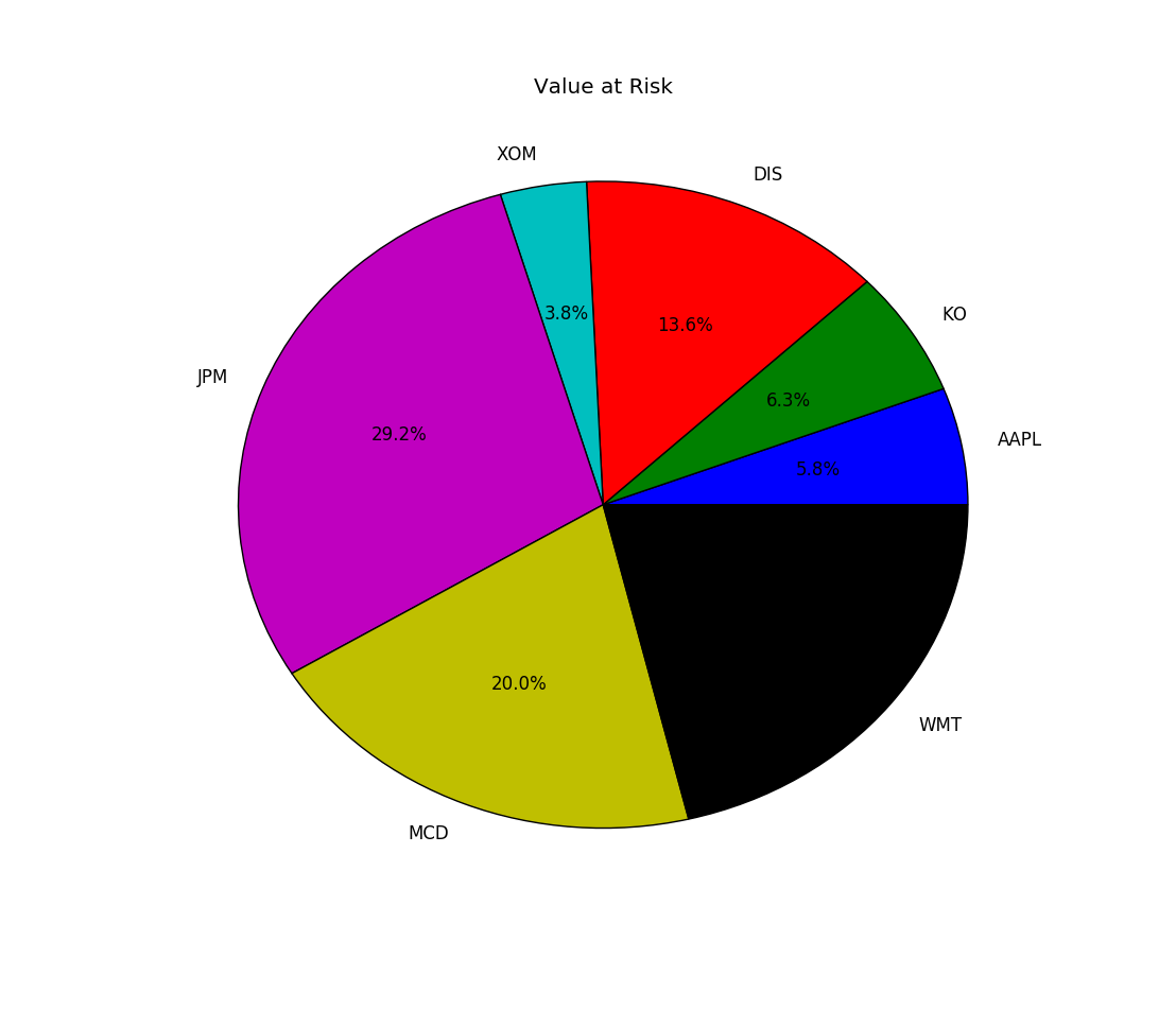
This post discusses the Value at Risk (VaR) measure used in financial markets, including the variance-covariance method, marginal VaR, component VaR, and then analyze the risk profile of a real portfolio.

Introduction

Value at Risk (VaR) is widely used by financial institutions to measure market risks or potential investment losses. It tells the maximum possible loss for a given portfolio over a certain time horizon, with a certain confidence level \(\alpha\), or

\[ Pr(Loss \le -VaR)=1-\alpha \tag{1.1} \]

There are three approaches to calculate VaR, that is, historical simulation, variance-covariance, and Monte Carlo simulation.

If you have difficulty viewing the formulas, right click on it and select Math Settings Math Renderer to switch to another format.

In this post we explore the variance-covariance method, or the delta-normal method, for VaR, Marginal VaR, and Component VaR. Consider a portfolio of n assets with corresponding weights w and covariance matrix \(\Sigma\), then the value this portfolio V, and its return and risk are

\[ \begin{matrix} V&=&\sum_{i=1}^{n} V_i\\ r_p&=& w^T\cdot r \\ \sigma_p^2 &=& w^T\Sigma w \end{matrix} \tag{1.2} \]

Assuming return normality, The value at risk of the portfolio in dollar amount is

\[ VaR_p = z\sigma_pV \tag{1.3} \]

where z is the inverser normal of confidence level \(\alpha\). For example, if \(\alpha\)=5%, then z=NORMSINV(0.95)=1.645 by Excel spreadsheet. Similarily, we can look at each individual stock and define its value at risk. Due to portfolio diversification, the portfolio VaR will be smaller than the sum of each individual VaR.

\[ \begin{matrix} VaR_i=z\sigma_i V_i \\ VaR_p \lt \sum_{i=1}^{n} VaR_i \end{matrix} \tag{1.4} \]

A natural question then is if we can normalize VaR so that the VaR of all the component stocks sum up to exactly the VaR of the portfolio? This is the concept of Marginal VaR (MVaR) and Componenet VaR (CVaR).

Marginal VaR is defined as derivative of portfolio w.r.t the per unit dollar change in value of the component stock, or

\[ MVaR_i=\frac{\partial VaR_p}{\partial V_i} = \frac{\partial z\sigma_pV_p}{\partial w_iV_p}=z\frac{\partial \sigma_p}{\partial w_i}=z\frac{\sigma_{ip}}{\sigma_p} \tag{1.5} \]

where \(\sigma_{ip}\) is the covariance between ith asset and portfolio p, and the last equation uses the following fact that,

\[ \begin{matrix} \frac{\partial\sigma_P}{\partial w_i} &=& \frac{[ \sum_{i=1}^{n} w_i^2\sigma_i^2 + \sum_{i=1}^n \sum_{j=1, j\ne i}^{n} w_iw_jc_{ij} ]^{1/2} } { dw_i } \\\\ &=& \frac{1}{2} [ 2w_i\sigma_i^2 + 2 \sum_{j=1, j\ne 1}^{n} w_jc_{ij} ] \times [ \sum_{i=1}^{n} w_i^2\sigma_i^2 + \sum_{i=1}^n \sum_{j=1, j\ne i}^{n} w_iw_jc_{ij}]^{-1/2} \\\\ &=& \frac{w_i^2\sigma_i^2 + \sum_{j=1, j\ne 1}^{n} w_j c_{ij} } {\sigma_p} = \frac{c_{ip}}{\sigma_p} \end{matrix} \tag{1.6} \]

Note that return correlation and beta coefficient are respectively,

\[ \begin{matrix} \rho_{ip}=\frac{\sigma_{ip}}{\sigma_i\sigma_p} \\ \beta_{ip}=\frac{\sigma_{ip}}{\sigma_p^2} \end{matrix} \tag{1.7} \]

then Marginal VaR can be rewritten as

\[ MVaR_i=z\frac{\sigma_{ip}}{\sigma_p}=z\sigma_i\rho_{ip}=z\sigma_p\beta_{ip} \tag{1.8} \]

At last, Component VaR (CVaR) is defined as,

\[ CVaR_i=MVaR_i \cdot V_i \tag{1.9} \]

It holds nicely to the following relationship,

\[ \sum_{i=1}^{n}CVaR_i=\sum_{i=1}^{n}z\sigma_p\beta_{ip}w_iV=z\sigma_pV\{\sum_{i=1}^{n}w_i\beta_{ip}\}=VaR_p \tag{1.10} \]

Real Portfolio

To illustrate the VaR delta-normal model, we continue to use the portfolio in the post in portfolio optimization.

First, let's download historical data and estimate the covariance matrix from it

assets = ['AAPL',       # Apple
          'KO',         # Coca-Cola
          'DIS',        # Disney
          'XOM',        # Exxon Mobil
          'JPM',        # JPMorgan Chase
          'MCD',        # McDonald's
          'WMT']         # Walmart

holdings = [100,200,300,400,500,600,700]          # number of shares in each assets

# download historical data from quandl
hist_data = {}
for asset in assets:
    data = quandl.get('wiki/'+asset, start_date='2015-01-01', end_date='2017-12-31', authtoken='ay68s2CUzKbVuy8GAqxj')
    hist_data[asset] = data['Adj. Close']
hist_data = pd.concat(hist_data, axis=1)

Then we can calculate portfolio VaR, marginal VaR, and component VaR via equations (1), (3) and (4), respectively,

# calculate historical log returns
hist_return = np.log(hist_data / hist_data.shift())
hist_return = hist_return.dropna()

port_cov = hist_return.cov()             # portfolio covariance matrix
port_corr = hist_return.corr()           # portfolio correlation matrix

V_i = hist_data.iloc[-1] * holdings        # dollar value as of end_date
V_i = V_i.as_matrix()                        # convert to vector
V_p = V_i.sum()                          # dollar value of the portfolio

z = norm.ppf(0.95, 0, 1)                # z value
sigma_p = np.sqrt(np.dot(V_i.T, np.dot(port_cov.as_matrix(),V_i)))    # note it's in dollar amount
VaR_p = z * sigma_p                      # portfolio VaR

sigma_i = np.sqrt(np.diag(port_cov.as_matrix()))        # individual asset
VaR_i = z * sigma_i * V_i

cov_ip = np.dot(port_cov.as_matrix(), V_i)/V_p               # covariance
beta_i = cov_ip / (sigma_p*sigma_p/V_p/V_p)                  # beta
MVar_i = VaR_p/V_p*beta_i                                    # marginal var

CVaR_i = MVar_i * V_i                                        # component var
CVaR_i_df = pd.DataFrame(data=np.column_stack((V_i, V_i/V_p, CVaR_i, CVaR_i/VaR_p, beta_i)))
CVaR_i_df.index = assets
CVaR_i_df.columns = ['Position ($)', 'Position (%)','CVaR ($)','CVaR (%)', 'Beta']
print(CVaR_i_df)

The compoenet VaR results are printed out as

      Position ($)  Position (%)     CVaR ($)  CVaR (%)      Beta
AAPL       16923.0      0.057814   211.850987  0.058426  1.010597
KO         21502.0      0.073457   227.700358  0.062797  0.854889
DIS        32082.0      0.109601   493.220879  0.136025  1.241094
XOM        18352.0      0.062695   138.558105  0.038213  0.609499
JPM        86060.0      0.294004  1058.301425  0.291868  0.992734
MCD        59250.0      0.202414   726.546655  0.200373  0.989919
WMT        58548.0      0.200016   769.783563  0.212298  1.061405

We have chosen big companies with beta close to one. So their component VaRs are in line with their position weights.

DISCLAIMER: This post is for the purpose of research and backtest only. The author doesn't promise any future profits and doesn't take responsibility for any trading losses.