Simple Linear Regression

This post discusses the linear regression model, including simple linear regression and multiple linear regression, and its implementations in Python, specifically in Scikit-Learn library. It also serves as a basis for further discussions of more advanced linear regression models such as Bayesian linear regression.

Introduction

Linear Regression is the most frequently used statistical and machine learning technique. It tries to put a straight line between feature variables \(X\) and label variable \(y\) that best fits the dataset. In mathematical term, it can be expressed as

\[ y=X\beta+\epsilon \tag{1.1} \]

where \(\beta\) is the parameter vector that includes the constant intercept term and exposure coefficients to each feature variable \(x\in X\).

Least Square (OLS) provides a closed-form estimation of coefficient \(\beta\) called normal equation given as follows:

\[ \hat{\beta} = (X^TX)^{-1}X^Ty \tag{1.2} \]

In the case of linear regression, it is also Maximinum Likelihood Estimation (MLE).

If you have difficulty viewing the formulas, right click on it and select Math Settings Math Renderer to switch to another format.

There are tons of materials about this topic in textbooks and online so I won't spill out more formulas. Let's look at the Python code illustration.

Simple Illustration

First let's generate a sample dataset and then solve for the coefficient via the Normal equation

import numpy as np
import pandas as pd
import matplotlib.pyplot as plt

sample_size = 500
sigma_e = 3.0             # true value of parameter error sigma
random_num_generator = np.random.RandomState(0)
x = 10.0 * random_num_generator.rand(sample_size)
e = random_num_generator.normal(0, sigma_e, sample_size)
y = 1.0 + 2.0 * x +  e          # a = 1.0; b = 2.0; y = a + b*x
plt.scatter(x, y, color='blue')

# normal equation to estimate the model parameters
X = np.vstack((np.ones(sample_size), x)).T
params_closed_form = np.linalg.inv(X.T.dot(X)).dot(X.T).dot(y)
print('pamameters: %.7f, %.7f' %(params_closed_form[0], params_closed_form[1]))

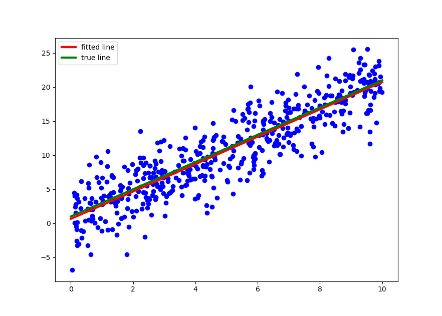
The coefficient and intercept used to generate the dataset are 2.0 and 1.0. Then when we try to back out them from the dataset we get 2.0086851 and 0.6565181, respetively. This is within the confidence interval of regression statistics.

Nevertheless there is no need to solve for the coefficent directly, as the recommended way to do so in Python is through its sklearn package.

from sklearn.linear_model import LinearRegression
# The next two lines does the regression
lm_model = LinearRegression(copy_X=True, fit_intercept=True, normalize=False)
lm_model.fit(x.reshape(-1,1), y)        # fit() expects 2D array
print('pamameters: %.7f, %.7f' %(lm_model.intercept_, lm_model.coef_))

# present the graph
xfit = np.linspace(0, 10, sample_size)
yfit = lm_model.predict(xfit.reshape(-1,1))
ytrue = 2.0 * xfit + 1.0       # we know the true value of slope and intercept
plt.scatter(x, y, color='blue')
plt.plot(xfit, yfit, color='red', label='fitted line', linewidth=3)
plt.plot(xfit, ytrue, color='green', label='true line', linewidth=3)
plt.legend()

# R-Square
r_square = lm_model.score(x.reshape(-1,1), y)
print('R-Square %.7f' %(r_square))

from scipy.stats.stats import pearsonr
# The square root of R-Square is correlation coefficient
print('Its square root is Pearson correlation coefficient: %.7f == %.7f' %(np.sqrt(r_square), pearsonr(x, y)[0]))

As you can see the true line and fitted line are hardly distingishable in the context of sample dataset. The R square indicates that 79.7% of the variability in y can be explained by x. Furthermore, in simple linear regression, its square root is Pearson correlation coefficient between \(x\) and \(y\), which shows 89% positive correlated.

Above is a quick introduction on linear regression, served as the starting point for more advanced topics in Machine Learning. Traditional topics such as multicollinearity, stepwise regression, generalized linear model, hierarchical linear model, and regularization methods such as lasso regression, ridge regression are not in my short-term plan. In next post we'll look at Beyesian Linear Regression.

Reference

DISCLAIMER: This post is for the purpose of research and backtest only. The author doesn't promise any future profits and doesn't take responsibility for any trading losses.