This post demonstrates how to perform a Bayesian linear regression, including the intuitions behind Bayesian statistics, linear regression Bayesian representation, conjugate Bayesian model, and Python implementation.
Introduction
In last post we reviewed the classical linear regression and now let's look from Bayesian perspective. There is well-known philosophical difference between frequentist and Bayesian. Interested readers can read further this debate online such as this one on Wiki. In my opinion, one advantage of Bayesian is its ability to perform online machine learning recursivelly as new information comes in incrementally.
In terms of the linear regression, Bayes's Theorem can be written as
\[ f(\beta|y,X)=\frac{f(y|\beta,X)f(\beta|X)}{f(y|X)} \tag{1.1} \]
where \(f(\beta|X)\) is the prior belief of parameter \(\beta\); \(f(y|\beta,X)\) is the likelihood of observing \(y\) given our prior; and \(f(y|X)\) is called evidence. Finally, \(f(\beta|y,X)\) is the posterior belief of pararmeter \(\beta\) once the evidence \(y\) has been taken into account. This posterior then becomes new prior and the circle continues recursively.
In this post we will bring the example from last post into Bayesian world.
If you have difficulty viewing the formulas, right click on it and select Math Settings Math Renderer to switch to another format.
Conjugate Bayesian Simple Regression
Let's continue to use the example from last post but re-phrase it in Bayesian way as follows
\[ y \sim N(X\beta, \sigma_eI) \\\\ \beta \sim N(\beta_0, \Sigma_{\beta,0}) \tag{2.1} \]
where the second formula claims that the prior distribution of parameter \(\beta\) is normal distribution with hyper-parameters \(\beta_0\) and \(\Sigma_{\beta,0}\); and the first formula says that the likelihood also follows a normal distribution. As you can see, the key step is to find the missing posterior distribution determined by Bayes Theorem.
To achieve this, we exploit a critical property known as conjugate prior in the Normal Inverse Gamma family. It mathematically proves that a normally distributed prior conjugates with normally distributed likelihood to produce a normally distributed posterior as
\[ \beta \sim N(\beta_1, \Sigma_{\beta,1}) \tag{2.2} \]
Now the question becomes to find new hyper-parameter \(\beta_1\) and its standard deviation \(\Sigma_{\beta,1}\).
Specifically in our previous example of simple linear regression,
\[ y=X\beta+\epsilon=a+bx+\epsilon \tag{2.3} \]
where \(a\) and \(b\) are intercept and slope, respectively. The hyper-parameters of prior are defined as
\[ \begin{matrix} \beta_0 &=& \begin{bmatrix} a_0 \\\\ b_0 \end{bmatrix} \\\\ \Sigma_{\beta,0} &=& \begin{bmatrix} \sigma_{a,0}^2 & 0 \\\\ 0 & \sigma_{b,0}^2 \end{bmatrix} \end{matrix} \tag{2.4} \]
if we observe two points \((x_1,y_1)\) and \((x_2, y_2)\) (it takes two points to determine a line), by using the Multivariate normal with known covariance matrix \(\Sigma\) (in our case two-points means bi-variate), the posterior is given as
\[ \begin{matrix} \beta_1 &=& \Sigma_{\beta,1}(\Sigma_{\beta,0}^{-1}\beta_0+\Sigma_y^{-1}\mu_y)\\\\ \Sigma_{\beta,1} &=& (\Sigma_{\beta,0}^{-1} + \Sigma_{y}^{-1})^{-1}\\\\ \mu_y &=& \begin{bmatrix} \frac{x_1y_2-x_2y_1}{x_1-x_2} & \frac{y_1-y_2}{x_1-x_2} \end{bmatrix}^T \\\\ \Sigma_{y} &=& \begin{bmatrix} [(\frac{x_1}{x_1-x_2})^2+(\frac{x_2}{x_1-x_2})^2]\sigma_e^2 & 0 \\\\ 0 & 2(\frac{1}{x_1-x_2})^2\sigma_e^2 \end{bmatrix} \end{matrix} \tag{2.5} \]
After that, \(\beta_1\), \(\Sigma_{\beta,1}\) become \(\beta_0\), \(\Sigma_{\beta,0}\) and the iteration continues.
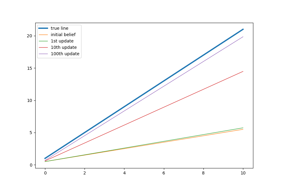
The formula seems complicated but conceptually it is very simple. Here is how it works. Imagine that in the beginning you believe the regression line should be horizontal. But then the first two points turn out to be vertical. So you think you might be wrong and you might not be so sure about things therefore you curved and tilt yourself toward the observed vertical line to somewhere 45 degrees. This is essentially what the above formulas do.
Then you continue to run another 249 time (because we have 500 points or 250 pairs). Everytime you adjust your previous belief by next two points you observe. It is easy to see that the longer you go, the less important it is where original starting belief is. Furthermore, there is nothing stopping you from reusing them again after you finish all the 500 points. It will make the estimation less and less dependent on the starting point and converges closer and closer to the true value.
As usual, here is the code implementation.
1
2
3
4
5
6
7
8
9
10
11
12
13
14
15
16
17
18
19
20
21
22
23
24
25
26
27
28
29
30
31
32
33
34
35
36
37
38
39
40
41
42
43
44
# don't forget to generate the 500 random samples as in the previous post
# initial belief
sigma_e = 3.0 # make it known to avoid inverse gamma complexity
a_0 = 0.5
b_0 = 0.5
sigma_a_0 = 0.5
sigma_b_0 = 0.5
beta_0 = np.array([[a_0], [b_0]])
sigma_beta_0 = np.array([[sigma_a_0*sigma_a_0, 0], [0, sigma_b_0*sigma_b_0]])
beta_recorder = [] # record parameter beta
beta_recorder.append(beta_0)
for pair in range(250): # 500 points means 250 pairs
x1 = x[pair*2]
x2 = x[pair*2+1]
y1 = y[pair*2]
y2 = y[pair*2+1]
mu_y = np.array([[(x1*y2-x2*y1)/(x1-x2)], [(y1-y2)/(x1-x2)]])
sigma_y = np.array([[(np.square(x1/(x1-x2))+np.square(x2/(x1-x2)))*np.square(sigma_e),0],
[0,2*np.square(sigma_e/(x1-x2))]])
sigma_beta_1 = np.linalg.inv(np.linalg.inv(sigma_beta_0)+np.linalg.inv(sigma_y))
beta_1 = sigma_beta_1.dot(np.linalg.inv(sigma_beta_0).dot(beta_0) + np.linalg.inv(sigma_y).dot(mu_y))
# assign beta_1 to beta_0
beta_0 = beta_1
sigma_beta_0 = sigma_beta_1
beta_recorder.append(beta_0)
print('pamameters: %.7f, %.7f' %(beta_0[0], beta_0[1]))
# plot the Beyesian dynamics
xfit = np.linspace(0, 10, sample_size)
ytrue = 2.0 * xfit + 1.0 # we know the true value of slope and intercept
plt.plot(xfit, ytrue, label='true line', linewidth=3)
y0 = beta_recorder[0][1] * xfit + beta_recorder[0][0]
plt.plot(xfit, y0, label='initial belief', linewidth=1)
y1 = beta_recorder[1][1] * xfit + beta_recorder[1][0]
plt.plot(xfit, y1, label='1st update', linewidth=1)
y10 = beta_recorder[10][1] * xfit + beta_recorder[10][0]
plt.plot(xfit, y10, label='10th update', linewidth=1)
y100 = beta_recorder[100][1] * xfit + beta_recorder[100][0]
plt.plot(xfit, y100, label='100th update', linewidth=1)
plt.legend()

That's all about Bayesian Linear regression. Nowadays we can import packages such as PyMC3 to solve it numerically without knowing the closed form details. But I still think it is useful to grasp the concepts by a simple example. Thanks for reading.
Reference
DISCLAIMER: This post is for the purpose of research and backtest only. The author doesn't promise any future profits and doesn't take responsibility for any trading losses.