Markov Chain Monte Carlo Linear Regression

This post discusses the Markov Chain Monte Carlo (MCMC) model in general and the linear regression representation in specific. MCMC is used to simulate posterior distribution when closed-form conjugate distribution such as the one in the previous Bayesian linear regression post is not available.

Introduction

In last post we examined the Bayesian approach for linear regression. It relies on the conjugate prior assumption, which nicely sets posterior to Gaussian distribution. In reality, most times we don't have this luxury, so we rely instead on a technique called Markov Chain Monte Carlo (MCMC). One popular algorithm in this family is Metropolis–Hastings and this is what we are looking at today. Before we proceed, I want to point out that this post is inpsired by this article in R.

MCMC answers to this question: if we don't know what the posterior distribution looks like, and we don't have the closed form solution as given in equation (2.5) of last post for \(\beta_1\) and \(\Sigma_{\beta,1}\), how do we obtain the posterior distrubtion of \(\beta\)? Can we at least approximate it? Metropolis–Hastings provides a numerical Monte Carlo simulation method to magically draw a sample out of the posterior distribution. The magic is to construct a Markov Chain that converges to the given distribution as its stationary equilibrium distribution. Hence the name Markov Chain Monte Carlo (MCMC).

MCMC Simple Linear Regression

Back to our simple linear regression example, firstly let's repeat the Bayesian Theorem from last post.

\[ f(\beta|y,X)=\frac{f(y|\beta,X)f(\beta|X)}{f(y|X)} \tag{2.1} \]

where \(\beta\) is regression parameter; y and X each have 500 observations.

The distribution of interest is our posterior distribution of \(\beta\) denoted as \(f(\beta|y,X)\). This time we technically only do one Bayesian iteration (remember we updated our belief 250 times in the last post?) because the purpose is to show how to draw a MCMC sample distribution from the first posterior iteration. We include all the 500 points in the Bayesian so the result is expected to reflect full information dataset and converge to the true value.

The Metropolis-Hastings algorithm works as follows.

1. Start with a random parameter value \(\beta_0\)
2. Choose a new \(\beta'\) based on some proposal function \(g(\beta'|\beta_0)\). As pointed out here, \(g\) must be symmetric, usually just Gaussian.
3. Calculate the acceptance ratio

\[ \alpha=\frac{f(y|\beta')f(\beta')}{f(y|\beta_0)f(\beta_0)} \tag{2.2} \]

4. Draw a random number \(u \in [0,1]\). Jump from \(\beta_0\) to \(\beta'\) if \(u <= \alpha\), and denote it as \(\beta_1\); otherwise stay with the old point.
5. Repeat step 2, 3, 4, and collect \(\beta_0\), \(\beta_1\),...,etc.

In the end, throw away some initial \(\beta\) values in the beginning based on burn-in hyper-parameter, and Metropolis-Hastings claims that the remaining \(\beta\) series comes from the distribution of posterior \(f(\beta|y,X)\).

Now let's interpret this process by code. There are Python packages such as PyMC3 to use out-of-box but sometimes it helps to look into the black box.

import scipy.stats
# don't forget to generate the 500 random samples as in the previous post
sigma_e = 3.0

# Similar to last post, let's initially believe that a, b follow Normal distribution with mean 0.5 and stadndard deviation 0.5
# it returns the probability of seeing beta under this belief
def prior_probability(beta):
    a = beta[0]     # intercept
    b = beta[1]     # slope
    a_prior = scipy.stats.norm(0.5, 0.5).pdf(a)
    b_prior = scipy.stats.norm(0.5, 0.5).pdf(b)
    # log probability transforms multiplication to summation
    return np.log(a) + np.log(b)

# Given beta, the likehood of seeing x and y
def likelihood_probability(beta):
    a = beta[0]     # intercept
    b = beta[1]     # slope
    y_predict = a  + b * x
    single_likelihoods = scipy.stats.norm(y_predict, sigma_e).pdf(y)        # we know sigma_e is 3.0
    return np.sum(np.log(single_likelihoods))

# We don't need to know the denominator of support f(y)
# as it will be canceled out in the acceptance ratio
def posterior_probability(beta):
    return likelihood_probability(beta) + prior_probability(beta)

# jump from beta to new beta
# proposal function is Gaussian centered at beta
def proposal_function(beta):
    a = beta[0]
    b = beta[1]
    a_new = np.random.normal(a, 0.5)
    b_new = np.random.normal(b, 0.5)
    beta_new = [a_new, b_new]
    return beta_new

# run the Monte Carlo
beta_0 = [0.5, 0.5]        # start value
results = np.zeros([50000,2])            # record the results
results[0,0] = beta_0[0]
results[0, 1] = beta_0[1]
for step in range(1, 50000):               # loop 50,000 times
    print('step: {}'.format(step))

    beta_old = results[step-1, :]
    beta_proposal = proposal_function(beta_old)

    # Use np.exp to restore from log numbers
    prob = np.exp(posterior_probability(beta_proposal) - posterior_probability(beta_old))

    if np.random.uniform(0,1) < prob:
        results[step, :] = beta_proposal    # jump
    else:
        results[step, :] = beta_old         # stay

burn_in = 10000
beta_posterior = results[burn_in:, :]
print(beta_posterior.mean(axis=0))        # use average as point estimates

# present the results
fig = plt.figure()
ax1 = fig.add_subplot(121)
ax1.hist(beta_posterior[:,0], bins=20, color='blue')
ax1.axvline(beta_posterior.mean(axis=0)[0], color='red', linestyle='dashed', linewidth=2)
ax1.title.set_text('Posterior -- Intercept')
ax2 = fig.add_subplot(122)
ax2.hist(beta_posterior[:,1], bins=20, color='blue')
ax2.axvline(beta_posterior.mean(axis=0)[1], color='red', linestyle='dashed', linewidth=2)
ax2.title.set_text('Posterior -- Slope')
plt.show()

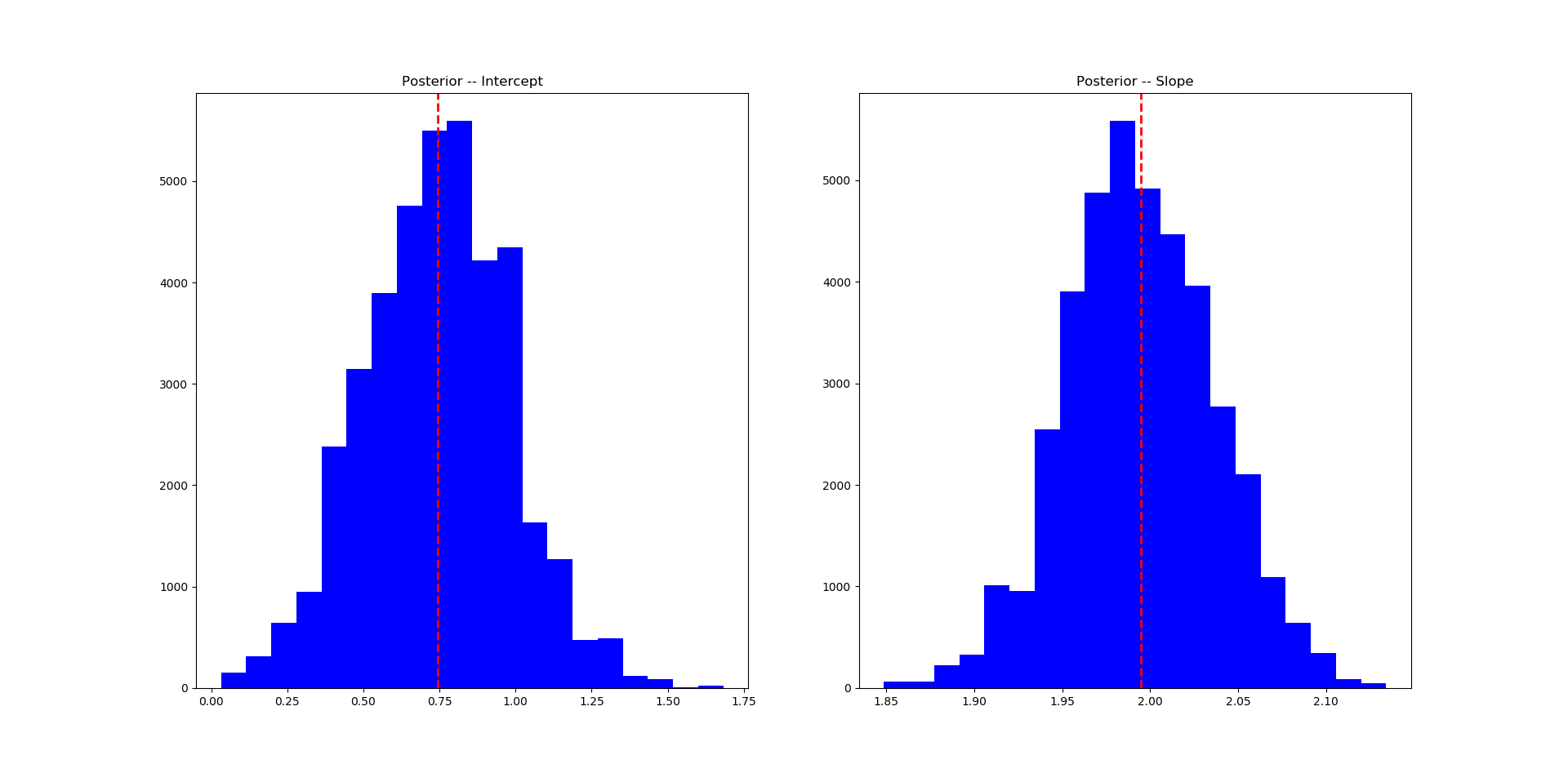
Here is the posterior distribution of \(\beta\). The intercept converges to 0.75 (linear regress gives 0.6565181) and the slope converges to 2 (linear regression gives 2.0086851). MCMC does the job.

Reference * Metropolis Hastings MCMC in R, 2010 * Metropolis Hastings Algorithm, Wikipedia

DISCLAIMER: This post is for the purpose of research and backtest only. The author doesn't promise any future profits and doesn't take responsibility for any trading losses.