Kalman Filter Linear Regression

In this post, we examine the linear regression model in the Kalman Filter world. It assumes that the underlying states are unobservable or partially observable, and Kalman Filter is designed to trace the latent state evolution through observations.

Introduction

Kalman Filter is a state space model that assumes the system state evolves by some hidden and unobservable pattern. Instead we can only observe some measurable features from the system, based on which we try to guess the current state of the system. An example would be without openning Bloomberg terminal, you try to guess stock market movement every day from the trader's mood. The graphical narrative can be found in this post.

This book provides a simple random walk example where the hidden state is the true equilibrium stock price in some time interval while stock close price of that interval serves as an observation with errors. Then it proves that the true equilibrium price is the weighted average of close prices with the weights being Fibonacci sequence. Dr Chan makes Kalman Filter popular to the online quantitative trading community with his EWA-EWC ETF pairs trading strategy.

In this post we will continue with our simple linear regression example from last post, and follow the plain Kalman Filter logic without the help of Python packages such as PyKalman.

Kalman Fitler Regression System

Kalman Filter as presented in the appendix is very mechanical. The hard part is to design a system that reflects the reality, and after that it's just a matter of following the mechanical steps.

In our simple linear example the state variable \(\theta\) contains intercept and slope and is assumed to follow a transition equation of random walk with Gaussian innovations:

\[ \theta_k = \begin{bmatrix} a_k \\\\ b_k \end{bmatrix} =\theta_{k-1} + w_t \tag{2.1} \]

where \(a_k\) and \(b_k\) are intercept and slope, respectively. This corresponds to equation \((A.1)\).

Comparing with last post where the posterior distribution is static, here the state evolves dynamically over time with linear transition conditions, hence the name Dynamic Linear Model (DLM).

After the state is transited, it's time to observe the system. Because it takes two points to determine a line, it is assumed to observe two points \((x_{1,t}, y_{1,t})\) and \((x_{2,t}, y_{2,t})\). The measurement equation \((A.2)\) can be re-written as,

\[ y_t =\begin{bmatrix} y_{1,t} \\\\ y_{2,t} \end{bmatrix}=\begin{bmatrix} 1 & x_{1,t} \\\\ 1 & x_{2,t}\end{bmatrix} \begin{bmatrix} a_t \\\\ b_t \end{bmatrix} + v_t \tag{2.2} \]

The last thing we need to start the system is the initial value \(\theta_{0|0}\) and \(P_{0|0}\)

After we've designed the system dynamics as above, the rest is to just follow the steps \((A.3)\) through \((A.9)\), which is done in the code as follows.

# don't forget to generate the 500 random samples as in the previous post
sigma_e = 3.0

# initial value
theta_0_0 = np.array([[0.5], [0.5]])         # 2x1 array
W = np.array([[0.5, 0], [0, 0.5]])          # 2x2 array
P_0_0 = W

results = np.zeros([250, 2])
for k in range(250):          # 250 pairs
    print('step {}'.format(k))
    # A-Priori prediction
    # first step, let k = 1
    theta_1_0 = theta_0_0
    P_1_0 = P_0_0 + W

    # After observing two points (x1, y1) and (x2, y2)
    x1 = x[2*k+0]
    x2 = x[2*k+1]
    y1 = y[2*k+0]
    y2 = y[2*k+1]
    y_1 = np.array([y1, y2]).reshape(2,1)
    F_1 = np.array([[1, x1], [1, x2]])
    y_1_tilde = y_1 - np.dot(F_1, theta_1_0)

    # residual covariance
    V_1 = np.array([[sigma_e, 0], [0, sigma_e]])
    S_1 = np.dot(np.dot(F_1, P_1_0), np.transpose(F_1)) + V_1

    # Kalman Gain
    K_1 = np.dot(np.dot(P_1_0, np.transpose(F_1)), np.linalg.inv(S_1))

    # Posterior
    theta_1_1 = theta_1_0 + np.dot(K_1, y_1_tilde)
    P_1_1 = np.eye(2) - np.dot(np.dot(K_1, F_1), P_1_0)

    # assign for next iteration
    results[k, :] = theta_1_1.reshape(2,)
    theta_0_0 = theta_1_1
    P_0_0 = P_1_1

print(results.mean(axis=0))     # intercept: 0.6694;   slope: 1.9926

# present the results
fig = plt.figure()
ax1 = fig.add_subplot(121)
ax1.plot(np.linspace(1, 250, num=250), results[:, 0])
ax1.title.set_text('Hidden State Evolution -- Intercept')
ax2 = fig.add_subplot(122)
plt.plot(np.linspace(1, 250, num=250), results[:, 1])
ax2.title.set_text('Hidden State Evolution -- Slope')
plt.show()

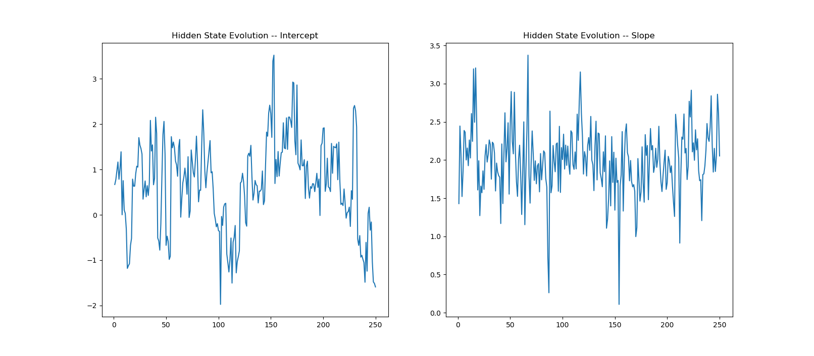
The results show average states are 0.6694 for intercept and 1.9926 for slope, pretty close to the linear regression results. The graph gives the evolution of states over the 250 observations.

Kalman Filter Linear Regression Hidden State Evolution

Reference

Appendix -- Mathematics

In this appendix we present a neat mathematical presentation of Dynamic Linear Model (DLM), following the notations in this book.

Firstly, The latent state transition is governed by the equation

\[ \begin{array}{lcl} \theta_t &=& G_t\theta_{t-1}+w_t \\\\ (p\times 1) & & (p\times p)(p\times 1)+(p\times 1) \end{array} \tag{A.1} \]

where \(w_t \sim i.i.d\hspace{5pt} N_p(0,W_t)\).

After state evolution, we have the measurement equation to observe it by

\[ \begin{array}{lcl} y_t &=& F_t\theta_t+v_t \\\\ (m\times 1) & & (m\times p)(p\times 1)+(m\times 1) \end{array} \tag{A.2} \]

where \(v_t \sim i.i.d.\hspace{5pt} N_m(0,V_t)\)

To kick off the system, we need initial guess of state variable \(\hat{\theta} _{0|0}\) and its initial covariance confidence matrix \(P _{0|0}\).

At each step \(k\), we first forecast a-priori predictions of state and state covariance as

\[ \begin{array}{lcl} \hat{\theta}_{k|k-1} &=& G_k\hat{\theta}_{k-1|k-1} \\\\ (p\times 1) & & (p\times p)(p\times 1) \end{array} \tag{A.3} \]

\[ \begin{array}{lcl} P_{k|k-1} &=& G_kP_{k-1|k-1}G_k^T+W_t \\\\ (p\times p) & & (p\times p)(p\times p)(p\times p)+(p\times p) \end{array} \tag{A.4} \]

Then after observing or measuring new \(y_k\), it's time to update our knowledge of the system by first calculating the innovation or measurement residual as how far away our forecast from the observation

\[ \begin{array}{lcl} \hat{y}_{k} &=& y_k-F_k\hat{\theta}_{k|k-1} \\\\ (m\times 1) & & (m\times 1)-(m\times p)(p\times 1) \end{array} \tag{A.5} \]

and residual covariance

\[ \begin{array}{lcl} S_k &=& F_kP_{k|k-1}F_k^T+V_k \\\\ (m\times m) & & (m\times p)(p\times p)(p\times m)+(m\times m) \end{array} \tag{A.6} \]

The Kalman gain reflects how much the residual contributes to the state update, is given by

\[ \begin{array}{lcl} K_k &=& P_{k|k-1}F_k^TS_K^{-1} \\\\ (p\times m) & & (p\times p)(p\times m)(m\times m) \end{array} \tag{A.7} \]

and Posterior estimation of state and state covariance

\[ \begin{array}{lcl} \hat{\theta} _{k|k} &=& \hat{\theta} _{k|k-1}+K_k\hat{y_k} \\\\ (p\times 1) & & (p\times 1)+(p\times m)(m\times 1) \end{array} \tag{A.8} \]

\[ \begin{array}{lcl} P_{k|k} &=& (I-K_kF_k)P_{k|k-1} \\\\ (p\times p) & & ((p\times p)-(p\times m)(m\times p))(p\times p) \end{array} \tag{A.9} \]

After this, repeat the steps between (A.3) and (A.9)

DISCLAIMER: This post is for the purpose of research and backtest only. The author doesn't promise any future profits and doesn't take responsibility for any trading losses.