This post shows how to use Tensorflow library to do linear regression. We can either use TF low-level API or high-level Keras API. The data is trained in batches and stochastic gradient descent backpropagation is used to estimate parameters such as intercept and slope. It is a long way compared with previously discussed classical linear regression methods, yet serves as a starting point to deep learning and reinforcement learning world.
Introduction
After four posts on linear regression, we are finally at the door of deep learning. Today we will build a simple feed-forward neural network (but not deep) with the help of Tensorflow to solve the linear regression problem. Tensorflow is a popular open-source deep learning library; the other popular choice is PyTorch .
Instead of defining graph and then executing in a session, Tensorflow 2.0 offers dynamic graph through eager execution. The code structure is completely different from 1.0, so we updated code here on Github.
We will try two implementations, one with low-level Tensorflow API and the other with high-level Keras API.
Low-Level API
Intuitively, Low-level API is more powerful and flexible, yet less efficient to develop. Here we set up a dataset pipeline with batch size 10. Then find gradient to this batch using automatic differentiation tape, and update slope and intercept with gradient descent. The code is as below.
1 | w = tf.Variable(tf.random.normal(shape=[1], dtype=tf.float64)) # scaler, shape=[] or shape=[1,] |
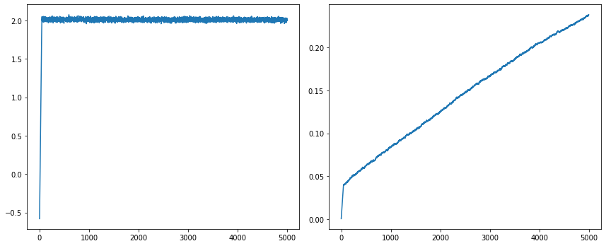
The results are 0.2377 and 2.0000 respectively. It's interesting to see that the slope quickly reaches 2.0 and stays there, while intercept gradually reaches 0.2377 at the end of training, and shows room for further improvements. This simple model is a good starting point for neural networks. It shows that the convergence depends on a lot of moving parts, including batch size, learning rate, initial values, etc. Rerun the notebook with modified settings will yield different results under limited epoch numbers. Although it shows the tendency of heading toward (1.0, 2.0) true values.

High-Level API
THe high-level API of Tensorflow is Keras, which now becomes part of Tensorflow. It has a couple of elements, a model, a loss function as objective, and an optimizer to reach that objective.
1 | loss_fn = tf.keras.losses.mean_squared_error |
We can manually use AutoDiff tape as before to train the model as,
1 | epochs = 200 |
On the other hand, as a high-level API, Keras model can be trained in one line,
1 | tf.keras.backend.clear_session() |
The results are 0.9672 and 1.9953, respectively. It suggests that we should use high-level APIs whenever possible; it is internally optimized to give better performance.
This code snippet scratched the surface of Tensorflow. Next step we are going to investigate a real deep neutral network called Long Short Term Memory (LSTM), which suits very well in financial time series analysis such as stock market forecast.
Reference * Géron, Aurélien. Hands-on machine learning with Scikit-Learn, Keras, and TensorFlow: Concepts, tools, and techniques to build intelligent systems. O'Reilly Media, 2019.
DISCLAIMER: This post is for the purpose of research and backtest only. The author doesn't promise any future profits and doesn't take responsibility for any trading losses.