This post discusses the basic practices of portfolio management and mean-variance portfolio optimization, including Efficient Frontier, Global Minimum Variance, Tangency Portfolio, and their implementations in Python.
Introduction
Modern Portfolio Theory (MPT) studies the tradeoff between return and risk. The risk of a portfolio is determined by not only the variance but also the correlations among assets. For a given risk, a rational investor would prefer an allocation with a higher expected returns; On the other hand, for a given return, he or she would prefer the portfolio with a lower risk level. This is a typical dual optimization problem.
This post examines the classic mean-variance portfolio optimization from computational mathematics' perspective, with mathematical formulas and programming codes. We will use real world stock data from Quandl.
Assume we have \(n\) assets and their expected return column vector is \(\mu\) and their covariance matrix is \(\Sigma\). Then the return and variance of a portfolio that invests in these n assets with weight \(w\) are, respectively,
\[ \begin{matrix} \mu_p &=& w^T\mu \\\\ \sigma_p^2 &=& w^T\Sigma w \tag{1.1} \end{matrix} \]
In addition, the covariance between two portfolios of respective weights \(w_1\) and \(w_2\), is
\[ \rho_{12}=cov(w_1^T\mu,w_2^T\mu)=w_1^T\Sigma w_2 \tag{1.2} \]
Let's illustrate this with some codes. First let's download the historical data.
1 | assets = ['AAPL', # Apple |
Here the historical window is set to be between 2015/01/01 and 2017/12/31 for the results to be reproducible. The return and correlation in this time range are as follows.
1 | # average daily return |
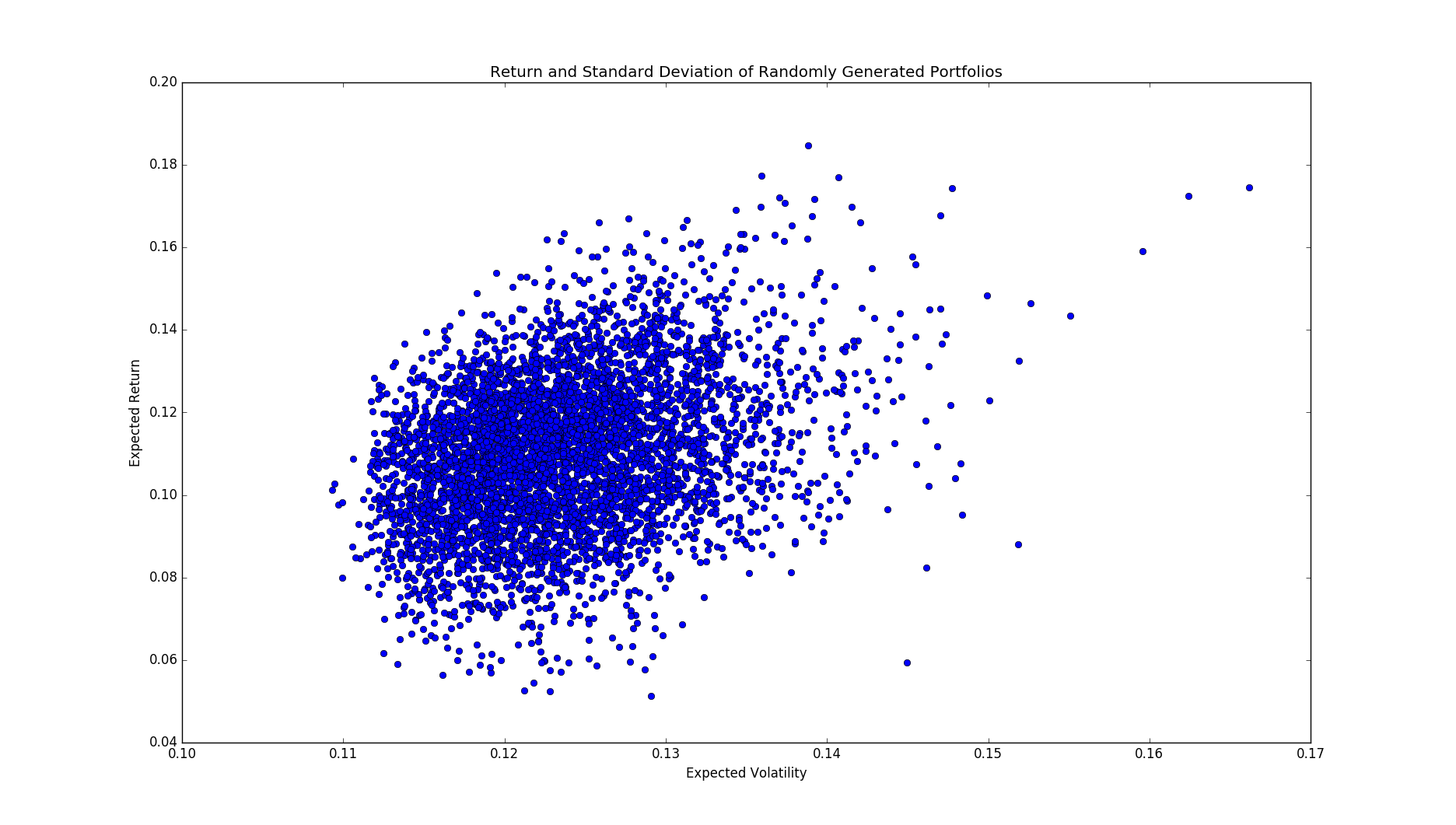
Now let's use Monte Carlo simulation to contruct 5,000 portfolios with random generated weights \(w\).
1 | # construct random portfolios |

As you can see, asset allocation makes a difference. Some portfolios are superior to others; achieving higher returns at the cost of lower risks. This is where the professional portfolio managers can add value to. So how to choose a good allocation? We will explore some basic solutions in the following sections.
Global Minimum Variance (GMV)
Of all the portfolios in figure 1, Global Minimum Variance (GMV) is the far left one. It is the lowest risk one can achieve by holding the seven stocks above. Mathematically, to find the Global Minimum Variance Portfolio, we need to solve
\[ \begin{matrix} \min & \sigma^2=w^T\Sigma w \\\\ s.t. & w^T\mathbf{1} = 1 \end{matrix} \tag{2.1} \]
The Lagrangian for this problem is
\[ L(w,\lambda)=w^T\Sigma w+\lambda(w^T\mathbf{1}-1) \tag{2.2} \]
and its first order condition is
\[ \begin{matrix} \frac{\partial L}{\partial w} &=&w^T(\Sigma +\Sigma^T)+\lambda \mathbf{1}^T &=& 0 \\\\ \frac{\partial L}{\partial \lambda} &=& w^T\mathbf{1} -1 &=& 0 \end{matrix} \tag{2.3} \]
To solve this system of two equations, first we solve for w from the first equation
\[ w = -\frac{1}{2}\lambda\Sigma^{-1}\mathbf{1} \tag{2.4} \]
Then we put it into the second equation to solve \(\lambda\),
\[ \begin{matrix} w^T\mathbf{1}&=&(-\frac{1}{2}\lambda \mathbf{1}^T\Sigma^{-1})\mathbf{1}=1 \\\\ &\Rightarrow& \lambda = -\frac{2}{\mathbf{1}^T\Sigma^{-1}\mathbf{1}} \end{matrix} \tag{2.5} \]
Finally substitute \(\lambda\) back to solve for the optimal \(w\)
\[ w^*=\frac{\Sigma^{-1}\mathbf{1}}{\mathbf{1}^T\Sigma^{-1}\mathbf{1}} \tag{2.6} \]
The following code snippet provides the close form solution via (2.6) 1
2
3
4
5
6
7
8
9# Global Minimum Variance (GMV) -- closed form
hist_cov_inv = - np.linalg.inv(hist_cov)
one_vec = np.ones(len(assets))
w_gmv = np.dot(hist_cov_inv, one_vec) / (np.dot(np.transpose(one_vec), np.dot(hist_cov_inv, one_vec)))
w_gmv_df = pd.DataFrame(data = w_gmv).transpose()
w_gmv_df.columns = assets
stdev_gmv = np.sqrt(np.dot(w_gmv.T, np.dot(hist_cov, w_gmv))) * np.sqrt(250)
print(w_gmv_df)
print(stdev_gmv)
Alternatively, we can use Python quadratic solver to solve (2.1) numerically. It should yield the same answer. Here we use the Python cvxopt package. For additional information, please refer to their online documentation and online example.
1 | # Global Minimum Variance (GMV) -- numerical |
Both methods yield the following optimal weights.
1 | # GMV weights |
Efficient Portfolio
To find an efficient portfolio other than GMV, we face a dual optimization problem. The primary problem finds highest return given a certain risk level \(\sigma_o\)
\[ \begin{matrix} \max & \mu_p=w^T\mu \\\\ s.t. & \sigma_p^2=w^T\Sigma w=\sigma_{o}\\ & w^T\mathbf{1}=1 \end{matrix} \tag{3.1} \]
while its dual finds the minimum risk given a certain return level \(\mu_o\)
\[ \begin{matrix} \min & \sigma_p^2=w^T\Sigma w \\\\ s.t. & \mu_p=w^T\mu=\mu_{o} \\\\ & w^T\mathbf{1} = 1 \end{matrix} \tag{3.2} \]
It is more common to solve the dual minimization problem (3.2), whose Lagrangian function is given by
\[ L(w,\lambda_1, \lambda_2)=w^T\Sigma w + \lambda_1(w^T\mu-\mu_o) + \lambda_2(w^T\mathbf{1}-1) \tag{3.3} \]
and its first order condition is
\[ \begin{matrix} 2\Sigma w + \lambda_1\mu + \lambda_2 \mathbf{1} &=& 0 \\\\ w^T \mu-\mu_o &=& 0 \\\\ w^T\mathbf{1} - 1 &=& 0 \end{matrix} \tag{3.4} \]
Similarily, from the first equation we have
\[ w=-\frac{1}{2}\lambda_1\Sigma^{-1}\mu-\frac{1}{2}\lambda_2\Sigma^{-1}\mathbf{1} \tag{3.5} \]
and put it into the last two equations to get the matrix format of \(\lambda=[\lambda_1;\lambda_2]\) as
\[ -\frac{1}{2}\begin{pmatrix} \mu^T\Sigma^{-1}\mu & \mu^T\Sigma^{-1}\mathbf{1} \\\\ \mu^T\Sigma^{-1}\mathbf{1} & \mathbf{1}^T\Sigma^{-1}\mathbf{1} \end{pmatrix} \begin{pmatrix}\lambda_1 \\\\ \lambda_2\end{pmatrix} = \begin{pmatrix}\mu_o \\\\ 1\end{pmatrix} \tag{3.6} \]
which yields
\[ \begin{matrix} \lambda &=&\begin{pmatrix}\lambda_1 \\\\ \lambda_2 \end{pmatrix}=-2A^{-1}y \\\\ A &=& \begin{pmatrix} \mu^T\Sigma^{-1}\mu & \mu^T\Sigma^{-1}\mathbf{1} \\\\ \mu^T\Sigma^{-1}\mathbf{1} & \mathbf{1}^T\Sigma^{-1}\mathbf{1} \end{pmatrix} \\\\ y &=& \begin{pmatrix}\mu_o \\\\ 1\end{pmatrix} \end{matrix} \tag{3.7} \]
In the end, substitute \(\lambda\) back to solve for the optimal w as
\[ \begin{matrix} w^*&=&-\frac{1}{2}\Sigma^{-1}B\lambda=\Sigma^{-1}BA^{-1}y \\\\ B&=&[\mu;\mathbf{1}] \end{matrix} \tag{3.8} \]
The following code finds minimum risk portfolio with a given return level \(\mu_o=max(\mu)\)
1 | # Maximum return -- closed form |
As an alternative, we can solve numerically 1
2
3
4
5
6
7
8
9# Maximum return -- numerical
P = matrix(hist_cov.as_matrix())
q = matrix(np.zeros((len(assets), 1)))
A = matrix(np.hstack([np.array(hist_mean),one_vec.reshape(len(assets),1)]).transpose())
b = matrix([mu_o,1])
w_max_ret_v2 = np.array(solvers.qp(P, q, A=A, b=b)['x'])
w_max_ret_df_v2 = pd.DataFrame(w_max_ret_v2).transpose()
w_max_ret_df_v2.columns = assets
print(w_max_ret_df_v2)
Both methods yield the following optimal weights.
1 | # max return weights |
Efficient Frontier
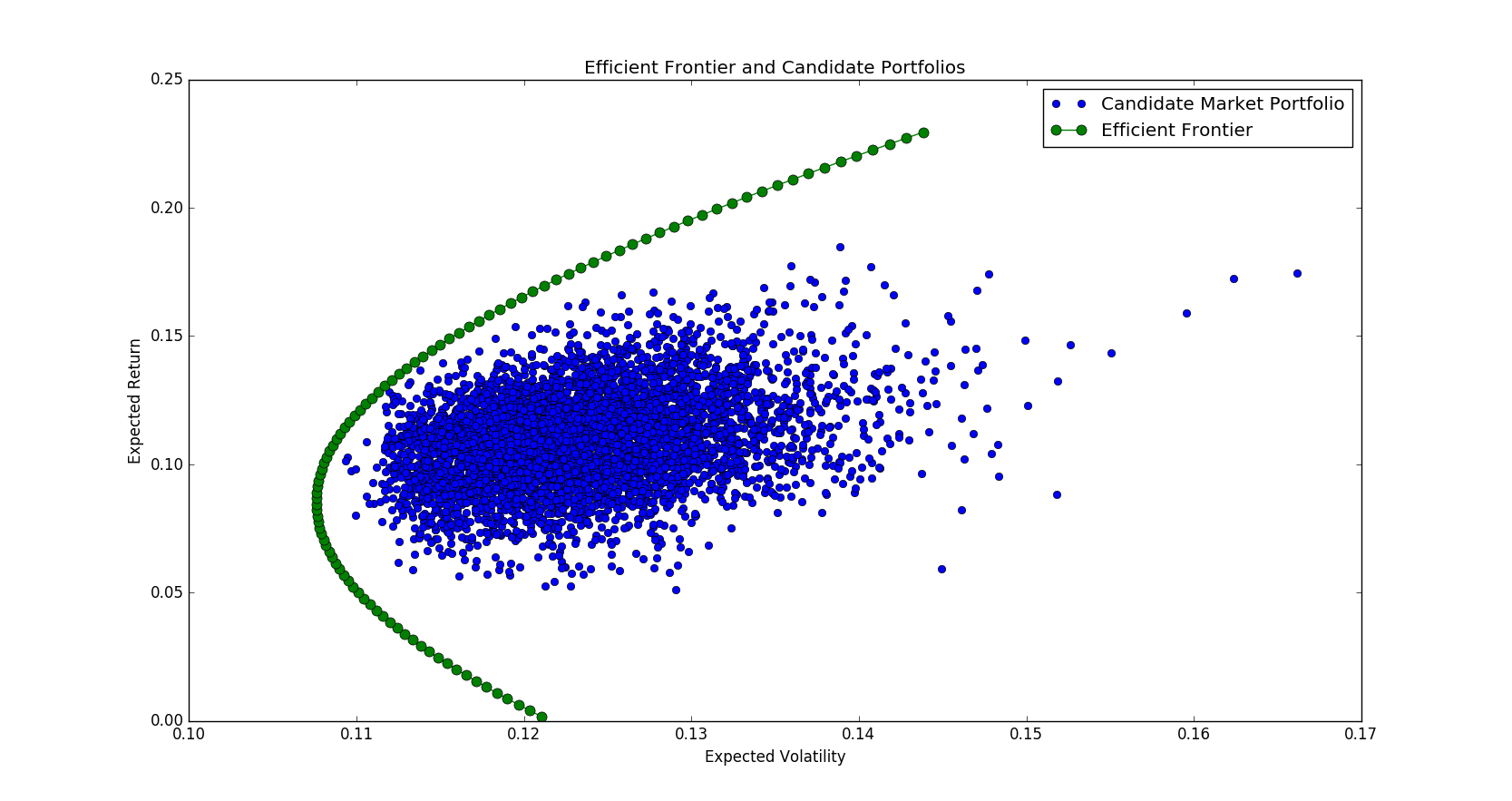
The previous section finds the minimum risk portfolio for a given return level. When we traverse all possible return levels, we get a set of optimal portfolios known as efficient frontier.
Alternatively, accordingly to Two_mutual_fund_theorem, it turns out we can construct the efficient frontier as a linear combination of the previous two portfolios, GMV and maximum return.
The code is similar to previous section except for a loop to traverse N target returns.
1 | # efficient frontier |

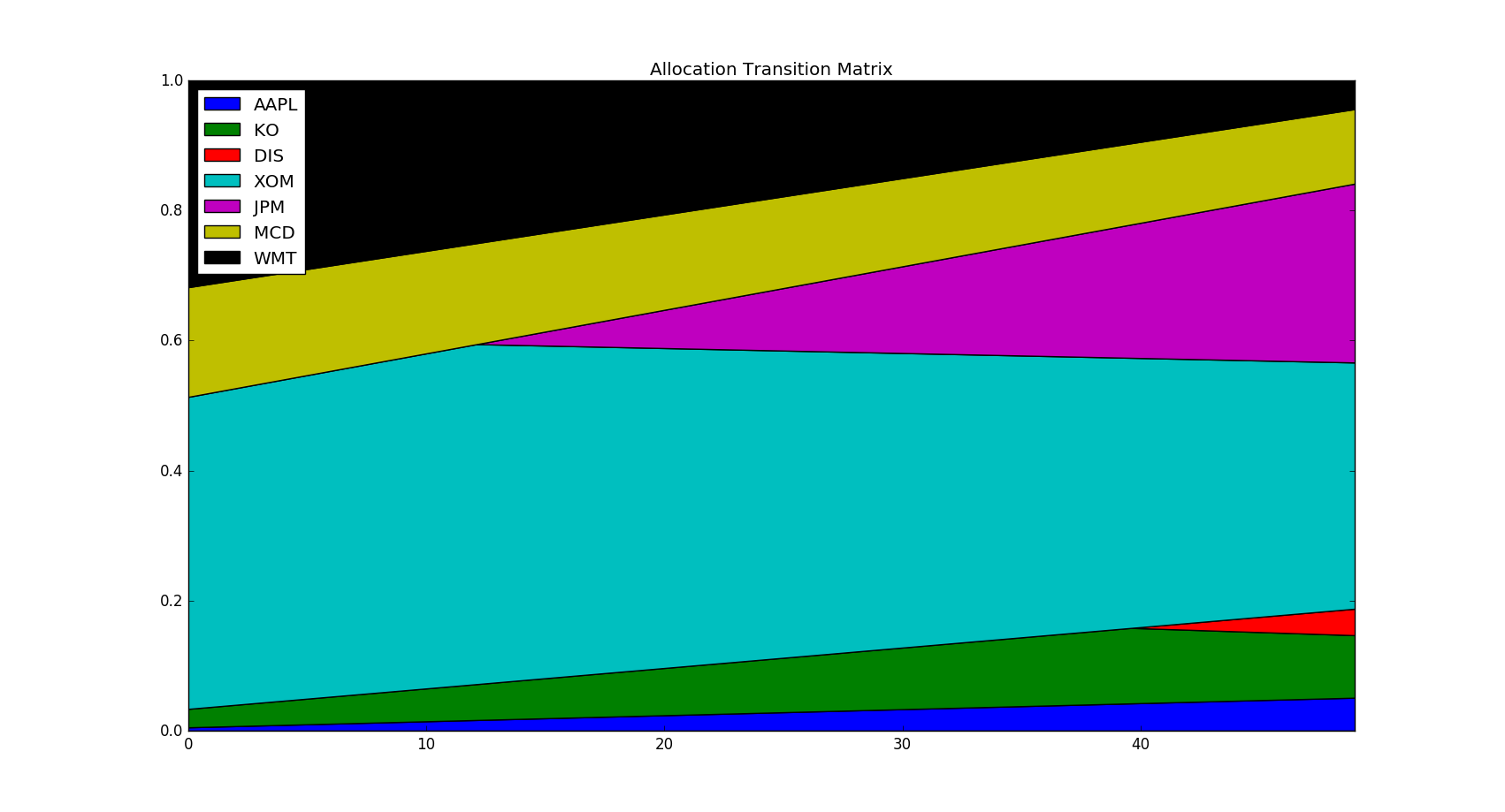
We can visualize the weight allocation transition matrix of efficient portfolios from low returns to high returns.
1 | transition_data = pd.DataFrame(optimal_weights) |

The transition figure tells us that for low returns it suffices to hold only five stocks. As we demand higher and higher returns, we start to hold JPM and then DIS.
Tangency Portfolio
Another interesting portfolio is tangency portfolio that maximizes Sharpe Ratio, one of the most popular measures for performance evaluation.
Denote risk free interest rate as \(r_f\), tangency portfolio targets the following equation,
\[ \begin{matrix} \max & \frac{\mu_p-r_f}{\sigma_p} = \frac{w^T\mu-r_f}{(w^T\Sigma w)^{\frac{1}{2}}} \\\\ s.t. & w^T\mathbf{1}=1 \end{matrix} \tag{5.1} \]
Because of the denominator, solve it directly via Lagrangian would be complicated. Fortunately we can be a bit creative and actually take advantage of the division format. Here is the intuitive approach. First, note that the ojective function is invariant with respect to leverage. In other words, it remains the same if we double the weight \(w\). Therefore the contraint can be ignored as long as \(w\) will be normalized in the end.
Secondly, if we knew the expected return \(r_o\) of the tangent portfolio, it must satisfy the following:
\[ \begin{matrix} \max & w^T\Sigma w \\\\ s.t. & w^T(\mu-r_f\mathbf{1})=r_o \end{matrix} \tag{5.2} \]
Solving this similarily to the previous section, it gives
\[ w=\frac{r_0}{(\mu-r_f\mathbf{1})^T\Sigma^{-1}(\mu-r_f\mathbf{1})}(\Sigma^{-1}(\mu-r_f\mathbf{1})) \tag{5.3} \]
By normalizing it, the arbitrary target expected return \(r_o\) actually goes away, leaving the optimal allocation as
\[ w^*=\frac{\Sigma^{-1}(\mu-r_f\mathbf{1})}{\mathbf{1}^T\Sigma^{-1}(\mu-r_f\mathbf{1})} \tag{5.4} \]
1 | # Maximum sharpe -- closed form |
Alternatively, we can use scipy package to solve numerically equation (5.1)
1 | from scipy.optimize import minimize |
Again they yield the same weights and sharpe ratio.
1 | # optimal weights |
We will revisit the tangible portfolio in the future section of CAPM. The figures will make more sense once no short sale constraint is added.
Reference
- Asset Pricing -- John Cochrane
- Python for Finance Second Edition -- Yuxing Yan
- Maximum Sharpe Portfolio in R -- Michael Kapler
DISCLAIMER: This post is for the purpose of research and backtest only. The author doesn't promise any future profits and doesn't take responsibility for any trading losses.