This post shows how to apply Kalman Filter in pairs trading. It updates the cointegration relationship using Kalman Filter, and then utilize this relationship in a mean-reversion strategy to backtest the pairs trading performance.
Introduction
In previous post we have seen Kalman Filter and its ability to online train a linear regression model. In last post we have also seen the idea of cointegration and pairs trading. As pointed out at the end of last post, one way to avoid look-ahead bias and gain walk forward analysis is through Bayesian online training mechanism such as Kalman Filter. Today we'll apply this idea to pairs trading.
As usual, the backtest codes in this post is located here on Github.
Pairs Trading via Kalman Filter
The idea is simple. Because we can obtain pairs trading hedge coefifcient through linear regression, and linear regression can be solved by Kalman Filter as in this post, therefore we can link the pairs through Kalman Filter. In this post we are going to use PyKalman package, so the only thing you need to do is to understand the concept and then express the problem in Bayesian format. Let's inherit the notations from previous post (refer to as Prev).
The state variables are still the intercept \(a_k\) and the slope \(b_k\) as in Prev\((2.1)\). But this time let's observe one \(y_t\) a time. So Prev\((2.2)\) is re-written as
\[ y_t=[1,x_t]\begin{bmatrix} a_t \\\\ b_t \end{bmatrix}+v_t \tag{2.1} \]
If we consider the case EWA as indepedent variable \(x\) and EWC as depedent variable \(y\), then the setting corresponds to
\[ \begin{array}{lcl} G_t &=&I \\\\ \theta_t&=&\begin{bmatrix} a_t \\\\ b_t \end{bmatrix} \\\\ F_t&=&[1,x_t] \end{array} \tag{2.2} \]
in Prev\((A.1)\) and Prev\((A.2)\). Notice that the observation matrix \(F_t\) changes everytime with new EWA price \(x_t\).
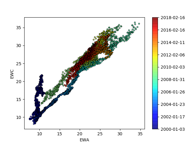
The following code explorer the relationship betwen EWA and EWC as a scatterplot colored by time.
1 | cm = plt.get_cmap('jet') |

From the scatterplot we can tell that their relationship changes between year 2010 and 2018. Therefore, the hedge ratio changes over time and our strategy needs to adapt to it. Otherwise using a static hedge ratio from linear regression would result in over- or under- hedge.
That is when Kalman Filter comes in to help. This time instead of do it manually, let's model Kalman filter with the help of pykalman package.
1 | # observation matrix F is 2-dimensional, containing sym_a price and 1 |
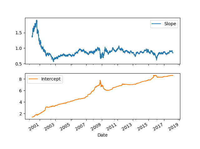
The code above is well commented. First fill in every input parameters based on your model design, and then just call kf.filter function to perform Kalman Filter. Note that the results are sensitive to your inputs such as your belief on observation_covariance and transition_covariance because they don't get adjusted over time.

From the figure above it seems slope between EWA and EWC is pretty stable around \(0.85\).
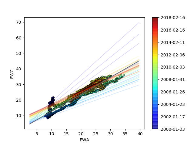
We can see how the regression line evolves over time, and relative to the line in black, which is the OLS line fitted to the whole dataset.

Last but not least, above codes work correctly but if we want to use Kalman filter in practce we have to take a different approach. That is, we want it to be updated step by step. Fortunately PyKalman also prvoides a function called kf.filter_update that serves this purpose. The code is a bit too long to fit here so I relegate it on github. You are encouraged to run it to see the equivalence but the latter allows for model updates every day upon new EWA and EWC prices, which will in turn be used in the next section.
Pairs Trading Backtest
It is time to backtest the EWA-EWC pairs trading on the Bollinger-bands strategy via Kalman Filter updates. The strategy is the same as last post. This allows us to compare the results with simple linear regression.
There is one thing needs to be pointed out in order to better understand the code, that is, the measurement error given in Pre\((A.5)\) is actually the spread at time k. To see this, notice that the first item on the right-hand side, \(y_k\), is the EWC price, and the second item,
\[ F_k\hat{\theta}_{k|k-1}=a_k+b_k*x_k \tag{3.1} \]
is the hedge side of EWA.
By the same logic, Pre\((A.6)\) is the variance of spread. In addition, Pre\((A.2)\) assumes the spread/eror term is normally distributed with zero mean and variance of Pre\((A.6)\). Therefore Pre\((A.5)\) and Pre\((A.6)\) provide the moving average and moving standard deviation (as sqaure root of variance) for Bollinger bands.
Unfortunately PyKalman package doesn't return them directly so we have to calculate them manually in the strategy. Here is the trading logic (also see [1]). Full code can be found here on github.
- On each day, observe EWA price \(x_t\) and EWC price \(y_t\)
- Calculate Pre\(A.5\) and Pre\(A.6\) as current spread and its variance
- Let Bollinger band be \(\hat{y}_{k}\pm\delta\sqrt{S_k}\)
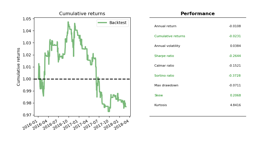
The backtest result is shown as follows. It seems the strategy was good until year 2017.

Reference * [1] Chan, Ernie. Algorithmic trading: winning strategies and their rationale. Vol. 625. John Wiley & Sons, 2013.
[2] Haohan Wang, 2015. Kalman Filters and Pairs Trading 1
[3] Haohan Wang, 2015. Kalman Filters and Pairs Trading 2
[4] Halls-Moore, M. (2014). Backtesting An Intraday Mean Reversion Pairs Strategy Between SPY And IWM
[5] Halls-Moore, M. (2016). Dynamic Hedge Ratio Between ETF Pairs Using the Kalman Filter
[6] Quantopian, David Edwards. Example: Kalman Filter Pairs Trade
DISCLAIMER: This post is for the purpose of research and backtest only. The author doesn't promise any future profits and doesn't take responsibility for any trading losses.