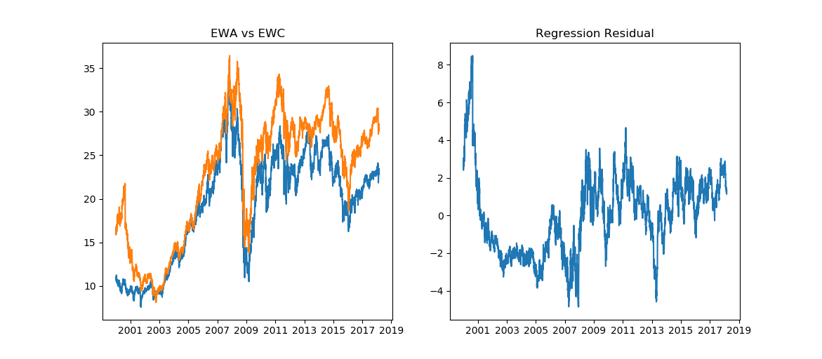
This post discusses stock pairs trading, including how to identify pairs or cointegration relationship using statistical tests, how to estimate the two-step error-correction model, and then backtests a pairs trading strategy in python.
Introduction
In last post we examined the mean reversion statistical test and traded on a single name time series. Often times single stock price is not mean-reverting but we are able to artificially create a portfolio of stocks that is mean-reverting. If the portfolio has only two stocks, it is known as pairs trading, a special form of statistical arbitrage. By combining two cointegrated stocks, we can construct a spread that is mean-reverting, even when these two stocks themselves are not. Please refer to the appendix if you want to check out cointegration first.
Cointegration and correlation talk abouot different things. For example, if two stock prices follow two straight lines with differennt slopes, then they are positively correlated but not cointegrated, as illustrated in this quora post. The mathematical formulas are relegated in the appendix.
The backtest codes in this post is located on Github.
Statistical Testing
Let's look at Ernie Chan's ([2]) EWA and EWC trade. The reasoning behind this trade is that both Canada and Australia's GDP rely heavily on natural resources, therefore their stock market performance are expected to be correlated through natural resources' prices.

EWA and EWC visually appear to be highly correlated with pearson correlation coefficient of 95%. The residual seems mean-reverting. Let's verify it with statistical tests.
Cointegrated Augmented Dickey Fuller Test
In order to perform ADF test as in last post, we need to know the hedging ratio between the two stocks. Cointegrated Augmented Dickey-Fuller (CADF) test determines the optimal hedge ratio by linear regression against the two stocks and then tests for stationarity of the residuals. CADF is also known as Engle-Granger two-step method.
1 | import statsmodels.tsa.stattools as ts |
The result indicates that the calculated test statistic of -3.667, smaller than the 5% critical value of -2.86; the p-value is 0.00459. This means that we can reject the null hypothesis of unit root or no cointegration. In other words, we accept that EWA and EWC are cointegrated with the hedging ratio given by the linear regression.
One undesired feature of the ordinary least square is that it is asymmetric, by switching the dependent and independent variables it will result in a differnet hedging ratio. A common solution is to do both sides, and choose the one with most negative / statistically significant test-statistic.
1 | lm_model = LinearRegression(copy_X=True, fit_intercept=True, normalize=False) |
Because the second regression has test-statistic of \(-3.79<-3.667\), we use EWC as independent variable and EWA as dependent variable. The coefficient is \(0.8328531\).
Johansen Test
It's understandable that if we do the test in two steps like in CADF, error accumulates between steps. Johansen test overcomes this by allowing us find hedge ratio and test cointegration at the same time. Another advantage of Johansen test is that it can be extended to more than two stocks.
Johansen test checks the rank \(r\) of \(\Pi\) in equation (A6). It gives statistical significance for \(r=0,1,2,...,n-1\) sequentially, where \(n\) is the full rank. The null hypothesis of \(r=0\) means no cointegration relationship; \(r \leq 1\) means up to one cointegration relationship, and so on. As a by product, the the eigenvectors of \(\Pi\) serves as hedge ratios for the stock portfolio.
1 | from statsmodels.tsa.vector_ar.vecm import coint_johansen |
From the test results above, we will reject null hypothesis of \(r=0\) easily. We can reject \(r\leq1\) up to 90% confidence level. There's another 10% of chance that \(r\) is 1 or based on (A6), they are cointegrated. It seems that Johansen test is more strict than the CDAF test regarding to accepting pairs. The first eigenvector can be normalized to \(-0.45169/0.534749=-0.84467\), which is pretty close to \(0.83285314\) from CADF section.
Pairs Trading
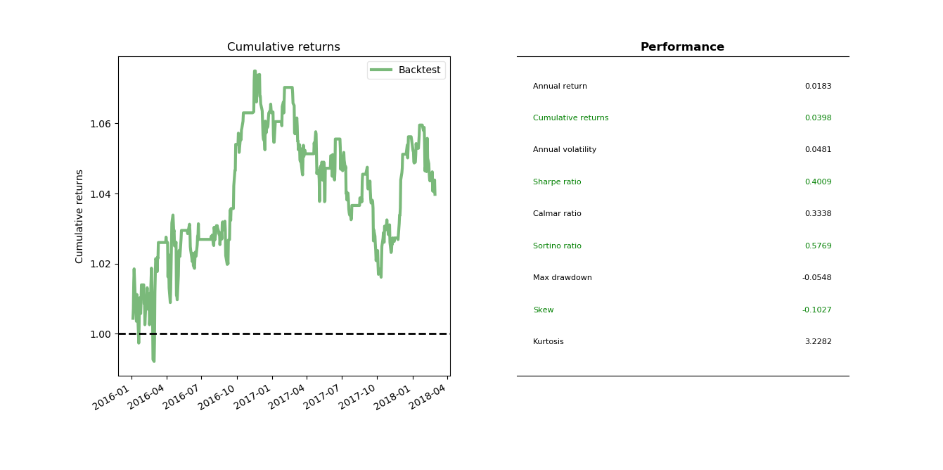
It is time to backtest the EWA-EWC pairs trading on the Bollinger-bands strategy. The strategy is very simple.
- Calculate the Bollinger bands as rolling moving average \(\pm\) scaler \(\times\) rolling standard deviation.
- If the spread touches upper band, short the spread; if the spread touches the lower band, long the spread.
- If the spread crosses the center line, flat the positions.
In order to avoid the look-ahead bias caused by using whole dataset for regression, we use a rolling window and re-estimate the linear regression at every step. This is also known as walk forward analysis. Another approach is to use online regression mechanism such as Kalman filter, which will be covered in the next post.
There are also two kinds of spreads: price spread and return spread. If B goes up $1 whenever A goes up $2, then buying 1 share of A and selling 2 shares of B becomes a price spread. If B goes up 1% whenever A goes up 2%, then buying $1 or \(1/P_A\) shares of A and selling $2 or \(2/P_B\) shares of B becomes a return spread. Because return spread in theory has to rebalance every day, here we use price spread.
The trading logic is posted below. Full code can be found here on github.
1 | if (spread[-1] > bollinger_ub) and (self.current_ewa_size >= 0): |

Appendix
Cointegration and Error-Correction Model
Cointegration loosely speaking means that two non-stationary time series can be paired up to form a stationary time series. Technically speaking it means there are more unit-root non-stationary components than the number of unit roots in the system. There are a lot of materials online about this topic but I found some of them hard for beginners to follow. In this appendix I try to convey the basic idea through an example.
Consider two time series
\[ \begin{aligned} y_{1t} &= y_{1,t-1}+b_{1,t}-0.5b_{1,t-1} \\ y_{2t} &= b_{2,t} \end{aligned} \tag{A1} \]
It is obvious \(y_{1t}\) is \(I(1)\) while \(y_{2t}\) is \(I(0)\) (see order of integration).
Now assume two stock prices \(x_{1t}\) and \(x_{2t}\) follows
\[ \begin{matrix} x_{1t} &=& 2y_{1t}+y_{2t} \\ x_{2t} &=& y_{1t}-2y_{2t} \end{matrix} \tag{A2} \]
By plugging \((A1)\) into \((A2)\), we get
\[ \begin{matrix} x_{1t} &=& x_{1,t-1}+2b_{1t}-b_{1,t-1}+b_{2t}-b_{2,t-1} \\ x_{2t} &=& x_{2,t-1}+b_{1,t}-0.5b_{1,t-1}-2b_{2t}+2b_{2,t-1} \end{matrix} \tag{A3} \]
Notice that both \(x_{1t}\) and \(x_{2t}\) are unit root non-stationary but both unit roots come from \(y_{1t}\) alone. In other words, there are two price series but there is only one unit root. \(x_{1t}\) and \(x_{2t}\) share a common trend \(y_{1t}\), and we can pair them up to cancel this common trend. Therefore \(x_{1t}\) and \(x_{2t}\) are said to be cointegrated. This is the mathematics behind the pairs trading.
From (A2), it's easy to find the pairing strategy as buying one lot of stock one and selling two lots of stock two,
\[ x_{1t}-2x_{2t}=5y_{2t} \]
In case we can't find it by eyes, we can use OLS to regress out the coeffficient, which is exactly what we did in the second section.
Last but not least, (A2) can be re-written as
\[ \begin{matrix} x_{1t}-x_{1,t-1}&=& -(0.2x_{1,t-1}-0.4x_{2,t-1})+2b_{1t}-b_{1,t-1}+b_{2t} \\\\ x_{2t}-x_{2,t-1} &=& (0.2x_{1,t-1}-0.4x_{2,t-1})+b_{1,t}-0.5b_{1,t-1}-2b_{2t} \end{matrix} \tag{A4} \]
or in VAR vector format
\[ \begin{matrix} \left[ \begin {array}{c} \Delta x_{1,t} \\\\ \Delta x_{2,t} \end{array} \right] &=&\left[ \begin {array}{c} -0.2 \\\\ 0.4 \end{array} \right]\left[ \begin {array}{cc} 1 & -2 \end{array} \right]\left[ \begin{array}{c} x_{1,t-1} \\ x_{2,t-1} \end{array}\right]+\left[ \begin{array}{c} 2b_{1t}-b_{1,t-1}+b_{2t} \\\\ b_{1,t}-0.5b_{1,t-1}-2b_{2t} \end{array}\right] \end{matrix} \tag{A5} \]
This is the well-known Engle and Granger (1987) Error-Correction representation. Notice that formula (A5) indicates stock one has a tendency to pull down (\(-0.2<0\)) and stock two has a tendency to pull up (\(0.4>0\)), when the distance between them (\(x_{1,t-1}-2x_{2,t-1}\)) becomes bigger.
The first term on the right-hand side of (A5) is referred to as error-correction term. Let
\[ \Pi=\left[ \begin {array}{c} -0.2 \\\\ 0.4 \end{array} \right]\left[ \begin {array}{cc} 1 & -2 \end{array} \right]=\begin{bmatrix} -0.2 & 0.4 \\\\ 0.4 & -0.8 \end{bmatrix} \]
Johansen test first estimates \(\Pi\) and then check if it is full rank. Particularly in this example it will find coefficent as \([1, -2]\) and rank = 1 (not full rank).
ECM two-step Approach
To estimate the model in two steps is because one-step regression upon differences will miss the long-term relationship. Consider a simple system \[ \begin{aligned} x_t&=x_{t-1}+u_t \\ y_t&=y_{t-1}+v_t \end{aligned} \]
If we know \(x\) and \(y\) have a long term relationship \(y=ax+\epsilon\), then \[ \Delta y_t = y_t-y_{t-1}=ax_t-y_{t-1}+\epsilon_t=a\Delta x_t+ \left(ax_{t-1}-y_{t-1}\right)+\epsilon_t \]
It is clear now that first step is to regression \(\left(ax_{t-1}-y_{t-1}\right)\) and then put that into the second step regression. Also note that this is to find the VAR representation in ECM format. To test for cointegration, it usually performs ADF test on residuals from first step regression.
Reference
[1] Tsay, Ruey S. Analysis of financial time series. Vol. 543. John Wiley & Sons, 2005.
[2] Chan, Ernie. Algorithmic trading: winning strategies and their rationale. Vol. 625. John Wiley & Sons, 2013.
[3] Vidyamurthy, Ganapathy. Pairs Trading: quantitative methods and analysis. Vol. 217. John Wiley & Sons, 2004.
DISCLAIMER: This post is for the purpose of research and backtest only. The author doesn't promise any future profits and doesn't take responsibility for any trading losses.