Introduction
This post considers time series mean reversion rather than cross-sectional mean reversion. Time series mean reversion processes are widely observed in finance. As opposed to trend following, it assumes that the process has a tendency to revert to its average level over time. This average level is usually determined by physical or economical forces such as long term supply and demand. Prices might deviate from that long term mean due to sentimental or short-term disturbances on the market but eventually will revert back to its intrinsic value.
A continuous mean-reverting time series can be represented by an Ornstein-Uhlenbeck process or Vasicek model in interest rate field, which is a special case of Hull-White model with constant volatility. It is also the continuous-time analogue of the discrete-time AR(1) process. I relegate the mathematical details to appendix.
To calibrate the OU process, there are generally two approaches based on formula (A9), i.e., the Least square and Maximum Likelihood Estimation. This document gives a good summary and comparison of results.
The backtest codes can be found on Github.
Statistical Testing
Comparing to backtesting, [1] made a valid point about the importance of statistical testing in that it consists of full information of the time series instead of just a number of completed trades dependent on chosen parameters. In addition, we can be more confident that a profitable strategy is not just based on luck if it passes statistical tests.
Augmented Dickey-Fuller Test
Augmented Dickey–Fuller test (ADF) detects if a time series contains unit root. Technically the name of unit root comes from the fact that the autoregressive polynomial has a root on the unit circle but basically it implies nonstationary.
Wikipedia and reference books have good coverage on the formulas so I just go with intuitions. Notice that Formula (A9) is a linear regression equation. Therefore the test essentially tests if \(1-\theta=1\) or \(\theta=0\), which becomes standard test for linear regression coefficients. If \(1-\theta\) doesn not equal to 1, \(\Delta x_t\) will depend on the current level of \(x_t\), and therefore not a random walk. All the other lagging \(\Delta x\) items listed on wikipedia are just controls for serial correlations.
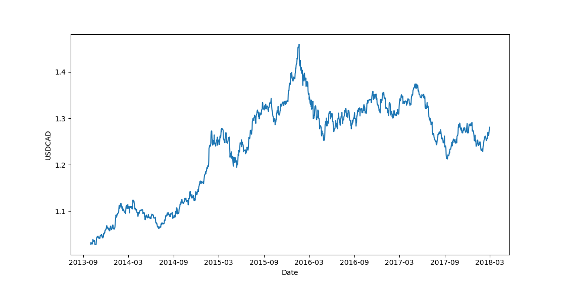
ADF test in Python is straightforward. Let's test historical USDCAD exchange rate,

1 | # ADF test |
Based on the results, we cannot reject the null hypothesis of \(1-\theta=1\). In other words, USDCAD contains unit root and is not mean reverting during this period. In fact, the figure above suggests an upward trend for USD, as Loonie lost about 30%.
Hurst Exponent
Another way of looking at stationarity is to compare it with Geometric Brownian Motion (GBM). A stationary price series is meant to diffuse more slowly than GBM. This is the theory behind Hurst exponent test. Considering GBM, the quadratic variation of its log value exhibits
\[ <|ln(S_{t+\tau})-ln(S_t)|^2>=\sigma^2\tau \sim \tau = \tau^{2H} \tag{2.1} \]
where \(\sim\) means proportional and \(H\) is Hurst Exponent. Apparently to make the last equation in (2.1) hold, H must be 0.5. Therefore we have the following rule for a price series,
- \(H<0.5\): mean reverting
- \(H=0.5\): geometric random walk
- \(H>0.5\): trending
Let's test the Hurst exponent on USDCAD prices.
1 | def hurst(ts): |
The Hurst function is adapted from QuantStart. The code logic is short and straightforward. From equation (2.1), if we take \(\tau=1,2,3,...\) etc, then the variance forms a straight line against this series of \(\tau\) values under GBM case. Therefore we can fit a regression line between them and use the slope to estimate Hurst exponent \(H\). One confusion one might have is that there is no variance calculation in the code. This comes from the fact variance and standard deviation (and square root) are log proportional, i.e.,
\[ ln(Var(Y))=ln(Std(Y)^2)=2ln(Std(Y)) \sim log(Std(Y)) \tag{2.2} \]
If you are interested in how many lags of \(\tau\) to be choosen, Robotwealth has a post to discuss the sensitivity of Hurst statistic on the choice of \(\tau\).
The Hurst statistic result \(0.555442813408275\) indicates USDCAD was in general (upward) trending during this time window.
Variance Ratio Test
Because of finite sample size, we need to know the statistical significance of Hurst statistic. In other words, we want a statistical test to tell us whether we can reject its null hypothesis of H equals 0.5. This hypothesis test is called Variance Ratio test ([1]).
1 | # (1.043812391881447, 0.23398177899239425, 0.5925003942830439) |
The code is credited to drtomstarke. It's a bit too long to fit into this article, so I save it to the source code on github repo.
The p-value says there is 59% chance that it is not a random walk.
Half-Life
The half life is calculated based on equation (A7); and use the estimated slope from (A8) as an approximate of \(\theta\).
1 | # half life |
It shows half life of 260 business days, roughly a year to come back half way toward its equilibrium level.
A linear scaling-in strategy
Inspired by [1], let's look at a simple linear mean-reversion strategy for USDCAD. The strategy is described as follows.
Use half-life as look-back window, find rolling mean and rolling standard deviation.
scaling-in and out by keep the posistiion size negatively porportional to the z-score.
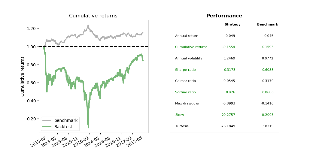
The following code is self-explanatory. It finds rolling z-score and then trades negatively proportional to it.
1 | def on_bar(self, bar_event): |

The benchmark is USDCAD exchange rate. It seems that between Oct-2015 and Jan-2016 when USD trending up, mean reversion strategies don't do well in their primitive settings. It came back right after until Apr-2016 when USD pulled back from 1.45 to 1.25. In the future we'll use Hidden Markov Chain to improve the performance by detecting if the market is in trending or mean-reverting phase.
The full code can be found in github repo.
Conclusion
In sum, this post considers one single time series. Next post we will look at two time series or pairs trading.
Reference
[1] Chan, Ernie. Algorithmic trading: winning strategies and their rationale. Vol. 625. John Wiley & Sons, 2013.
[2] Tsay, Ruey S. Analysis of financial time series. Vol. 543. John Wiley & Sons, 2005.
[4] QuantStart
Appendix A -- Stationarity
White noise
\[ \epsilon_t \sim N(0, \sigma^2) \]
is stationary.
Wiener process or Brownian motion (and its discrete version random walk) is not stationary, because covariance
\[ cov(W_s, W_t) = cov(W_s, W_s+W(t-s))=Var(W_s)=s \]
depends on \(s\).
ARMA process stationarity condition is that all roots reside outside of unit circle.
GARCH(1,1)
\[ \sigma_t^2=\omega+\beta \sigma_{t-1}^2 + \alpha \epsilon_{t}^2 \]
The conditional variance varies
\[ E_{t-1}[\sigma_t^2]=\omega + \beta \sigma_{t-1}^2 \]
But the unconditional variance
\[ \sigma = \frac{\omega}{1-\beta - \alpha} \]
is stationary if \(\alpha + \beta < 1\).
Appendix B -- Ornstein–Uhlenbeck process
An Ornstein–Uhlenbeck process is governed by the following stochastic differential equation
\[ dx_t=\theta (\mu-x_t)dt+\sigma dW_t \tag{A1} \]
With the help of Ito lemma, Wikipedia solves its solution as
\[ x_t = x_0e^{-\theta t}+\mu(1-e^{-\theta t})+\sigma \int_{0}^{t} e^{-\theta (t-s)}dW_s \tag{A2} \]
Therefore, its first two moments of its equilibrium distribution become
\[ E[x_t]=x_0 e^{-\theta t}+\mu(1-e^{-\theta t}) \rightarrow \mu \tag{A3} \]
\[ Var[x_t]=\frac{\sigma^2}{2\theta}(1-e^{-2\theta t})\rightarrow\frac{\sigma^2}{2\theta} \tag{A4} \]
It's half life is defined as the (expected) time to return half way to its mean, or
\[E[x(t_{0.5})]-\mu=\frac{x_0-\mu}{2} \tag{A5}\]
Then plus (A3) into (A5), the left-hand-side of (A5) becomes
\[ \begin{matrix} E[x(t_{0.5})]-\mu &=& x_0 e^{-\theta t_{0.5}}+\mu(1-e^{-\theta t_{0.5}})-\mu \\\\ &=& e^{-\theta t_{0.5}}(x_0-\mu) \end{matrix} \tag{A6} \]
Solving it with right-hand-side gives the half-life
\[e^{-\theta t_{0.5}}(x_0-\mu)=\frac{x_0-\mu}{2} \Rightarrow t_{0.5}=\frac{ln2}{\theta} \tag{A7}\]
It's obvious that the larger \(\theta\) is, the shorter is half life and thus stronger the mean-reversion effect.
The relationship with AR(1) can be seen by discretizing (A1)
\[ \Delta x_t=x_{t+1}-x_t=\theta\mu - \theta x_t +\delta \epsilon_{t_{i+1}} \tag{A8}\]
or in ARMA representation
\[ x_{t+1}=(1-\theta)x_t + \theta \mu + \delta \epsilon_{t_{i+1}} \tag{A9}\]
and the stationarity condition becomes
\[|1-\theta|<1 \rightarrow 0 < \theta < 2 \tag{A10}\]
Equation (A.10) also suggests that a mean-reversion process is not necessarily a stationary process (e.g. when \(\theta>2\)).
DISCLAIMER: This post is for the purpose of research and backtest only. The author doesn't promise any future profits and doesn't take responsibility for any trading losses.