This post demonstrates how to use Expecation-Maximization (EM) Algorithm, Gaussian Mixture Model (GMM) and Markov Regime Switching Model (MRSM) to detect the latent stock market regime switches.
Introduction
It's been a while since the post of Hidden Markov Chain (HMM), this time let's continue to explore some other popular regime switching models, including Gaussian Mixture model and Markov Regime Switching model (MRSM). Similar to HMM, the market regime is served as hidden states so they are all approached by some sort of Expectation-Maximization (EM) machine learning techniques. It's in place to have a brief discussion on EM algorithm first.
The accompanying notebook can be found here.
Expectation-Maximization
The simplest example on EM I can come up with has already been posted on stackexchange and the paper cited there. Here I will just make some comments on the coin-flipping example.
Maximum Likelihood Estimation (MLE) is the most widely used method to estimate model parameters. Yet it is only effective when the data generation process is transparent and there are no hidden or latent variables. In the example there are two coins with probability of heads \(\theta_A\) and \(\theta_B\) respectively, and we know exactly which coin generates the toss set (identified by blue and red). Then MLE estimation is simply the percentage of heads in the red and blue group, respectively.
If there exist latent variables, EM algorithm is used to find MLE estimation iteratively. In this case we don't know which coin is used to generate the toss set. The E-M two-step works as below. 1. E-step: make assumptions and complete the dataset Assume coin A gets head \(60\%\) of time, coin B \(50\%\) of time (or any other numbers you prefer). Had we picked coin A, the probability of seen first toss set (5H, 5T) is given by Binomial \[ \begin{pmatrix} 10 \\ 5 \end{pmatrix} (0.6)^5(0.4)^5=0.20 \]
simiarily the probability is \(0.246\) had we chosen coin B. Based on the likihoods, the probability of coin \(A\) behind the first toss set is \(0.20/(0.20+0.246)=0.45\) and \(1-0.45=0.55\) for coin \(B\), which makes sense because we would expect that it's more likely that coin \(B\) produced the toss set. Then (5H, 5T) contributes \(5H*0.45=2.2H\) to coin A, \(5H*0.55=2.8H\) to coin B, and so on the table on the right side.
- M-step: update the assumptions M-step is regular maximum likelihood estimation given the new probability table generated in the E-step.
Iterate step 1 and 2 until \(\theta_A\) and \(\theta_B\) converge.
Gaussian Mixture Model
In the above example, if we assume instead \(\theta_A\) and \(\theta_B\) come from two Gaussian distributions, respectively, then it becomes Gaussian Mixture model. A good illustration can be found here.
1 | from sklearn.mixture import GaussianMixture |

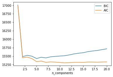
We may choose either two or three states based on the AIC graph. Two states could indicate high and low vol regimes; while three states hopefully can explain uptrend, downtrend and sideways. In this post we use two components. The result suggests first state is low vol (\(0.5\%\)), second state is high vol (\(5.6/%\)).
Markov Regime Switching Model
It's known that stock return is not normally distributed, having negative skewness and high kurtosis. It can be better modeled as conditional normal distribution (e.g. GARCH), which may suggest that the market can have different regimes and returns are normally distributed within a regime.
Here again we choose two regimes, and assuming return is centered around zero.
1 | from statsmodels.tsa.regime_switching.markov_regression import MarkovRegression |

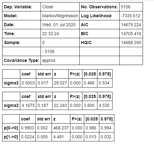
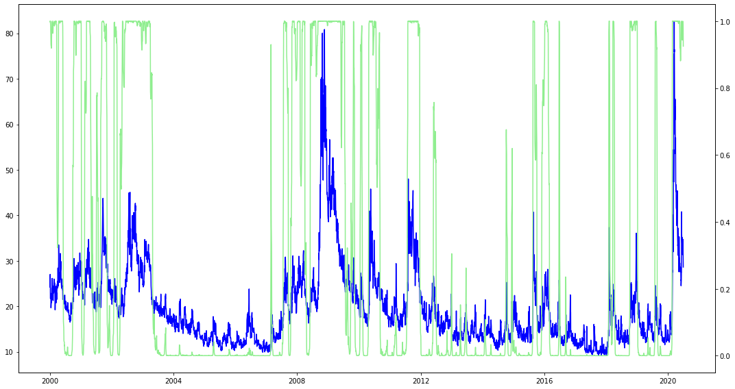
The result also suggests first state is low vol \(0.5\%\), while second state is high vol \(4.17\%\). By comparing the graphs, the regime switch model turns out to have better fit than Gaussian mixture; which is undertandable, because Gaussian mixture doesn't consider time sequence in time series. And comparing with VIX, Markov Regime Switching model captures major market downturns as shown below.

A straightforward way to use regime switching for trading is to assume regime doesn't change; or tomorrow is in the same regime as today.
Reference
VanderPlas, Jake. Python data science handbook: Essential tools for working with data. " O'Reilly Media, Inc.", 2016.
DISCLAIMER: This post is for the purpose of research and backtest only. The author doesn't promise any future profits and doesn't take responsibility for any trading losses.