This post discusses the AutoRegressive Integrated Moving Average model (ARIMA) and the Autoregressive conditional heteroskedasticity model (GARCH) and their applications in stock market prediction.
Introduction
An ARMA (AutoRegressive-Moving Average) has two parts, the AR(p) part and MA(q) part, expressed as below
\[ \begin{aligned} X_t &= c + \epsilon_t+\sum_{i=1}^p\varphi_iX_{t-i}+\sum_{i=1}^q\theta_i\epsilon_{t-i}\\\\ \left( 1-\sum_{i=1}^p\varphi_iL^i \right)X_t&=c+\left(1+\sum_{i=1}^q\theta_iL^i \right)\epsilon_i \end{aligned} \]
where \(L\) is the lag operator and \(\epsilon_i\) is white noise. It can be approached by Box-Jenkins method. We may use PACF plot to identify AR lag order \(p\), and ACF plot to identify MA lag order \(q\); or use information such as AIC and BIC to do the model selection.
ARIMA (AutoRegressive Integrated Moving Average) is a generalization of ARMA by adding an integrated part with order \(d\) for non-stationary processes.
While ARIMA works on price level or returns, GARCH (Generalized AutoRegressive Conditional heteroskedasticity) tries to model the clustering in volatility or squared returns. It extends ARMA terms to the variance front
\[ \begin{aligned} y_t&=x'_tb+\epsilon_t \;\;\; \epsilon_t \sim N(0, \sigma^2_t) \\\\ \sigma^2_t &= \omega + \sum_{i=1}^p \beta_i\sigma^2_{t-i}+\sum_{i=1}^q\alpha_i\epsilon^2_{t-i} \end{aligned} \]
As the discrete version of Stochastic Volatility model, GARCH also captures the fat-tail effect in stock markets. Therefore combining ARIMA with GARCH is expected to have a better fit in modelling stock prices than one model alone. In this post we will apply them to S&P 500 prices. The workbook can be found here.
ARIMA
First it's known that stock prices are not stationary; while returns mgiht be. This is confirmed by ADF unit root test.
1 | # price is known to be non-stationary; return is stationary |
ADF p-value for return series is \(0\), which rejects the null hypothesis of unit root. Therefore, we accept \(d=1\) in ARIMA(p, d, q), and the next step is to identify lag \(p\) and \(q\). The ACF and PACF plots suggest a lag up to \(35\) business days. There will be too many parameters to fit if we follow the graph. One solution is to use weekly or monthly charts. Here we constraint max lag to \(5\) days and use AIC to selct the best model.

1 | from statsmodels.tsa.arima_model import ARIMA, ARMA |
The next step is to fit the model and evaluate model fit through residual statistics. The residuals still show some autocorrelations, and didn't pass the normality tests. This is somehow expected, due to the lag order constraints.
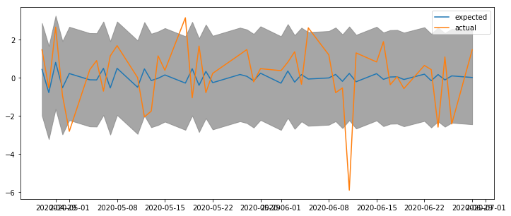
Nevertheless, let's proceed to the last step and use the model to forecast. Below it compares the return forecast on the test set and actual returns.

The return forecast is centered around \(0\%\), with confidence band between \(\pm2\%\). The outcome is not particularly impressive. After all, the market is undergoing a turbulent stage, even slumped \(6\%\) during the forecast time window.
GARCH
Let's see whether adding GARCH effect will yield a better result or not. The modelling process is similar to ARIMA: first identify the lag orders; then fit the model and evaluate the residual, and finally if the model is satisfactory, use it to forecast the future.
We constraint both the AR lag and GARCH lag be less than \(5\). The optimal order turns out to be \((4, 2, 2)\).
1 | from arch import arch_model |
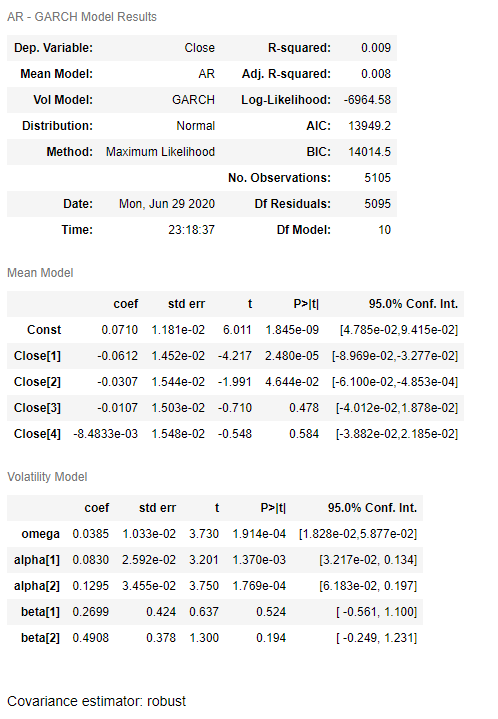
Next let's fit the model according to best parameters selected, as shown below. It confirms that the mean model is AR(4), and variance model is GARCH(2, 2). Some of the coefficients are not statistically significant.

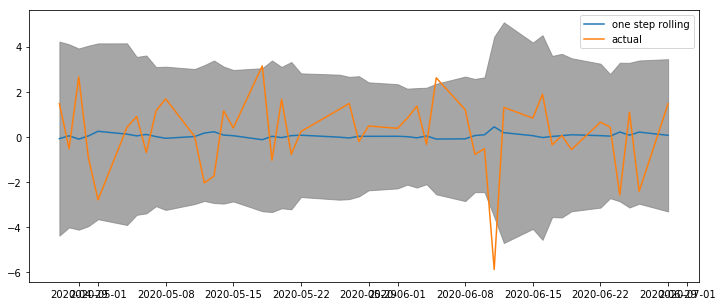
Last but not least, the forecast band fluctuates from \(\pm 4\%\) down to \(\pm 3\%\) before bounces back to \(\pm 5\%\), which clearly demonstrates volatility clustering as promised by the model. Note that here it is the one-step rolling forecast, and supposed to be better than the static multi-period forecast.

Appendix
Trend stationary and difference stationary Trend stationary, as known as deterministic trend, has deterministic mean trend. In contrast, difference stationary has stochastic trend. The former can be estimated with OLS, while the latter needs to be differenced first.
Consider a simple process \[ \begin{aligned} x_t &=at+u_t \\ u_t &= \varphi u_{t-1}+\epsilon_t \end{aligned} \]
If \(\varphi < 1\), the process is trend stationary; That is, if we substract trend \(at\), the process becomes stationary. If \(\varphi = 1\), it is difference stationary. It is easy to see the stochasticity by putting second equation into the first, and rewrite the equation as \[ x_t=at+(u_{t-1}+\epsilon_t)=a+x_{t-1}+\epsilon_t \]
DISCLAIMER: This post is for the purpose of research and backtest only. The author doesn't promise any future profits and doesn't take responsibility for any trading losses.